Advanced Modeling Topics
This section of notes will use the following packages.
library(modelr)
library(broom)
library(forcats)
library(stringr)
library(tidyverse)
Interactions
Interactions are an important modeling concept that can greatly increase model fit, prediction accuracy, and explained variance. Interactions can be difficult to interpret, however, we will explore them in more detail here with particular attention to graphical displays of interactions and also exploring the design matrix for how interactions are included in the model fitting procedure.
We will use the heights data from the modelr package to explore interactions. The primary interactions that we will explore are between two (or more) categorical predictors and also the interaction between a categorical predictor and a continuous predictor. Interpretations are similar between two continuous predictors as well.
Here are the first few rows of the data:
heights## # A tibble: 7,006 × 8
## income height weight age marital sex education afqt
## <int> <dbl> <int> <int> <fct> <fct> <int> <dbl>
## 1 19000 60 155 53 married female 13 6.84
## 2 35000 70 156 51 married female 10 49.4
## 3 105000 65 195 52 married male 16 99.4
## 4 40000 63 197 54 married female 14 44.0
## 5 75000 66 190 49 married male 14 59.7
## 6 102000 68 200 49 divorced female 18 98.8
## 7 0 74 225 48 married male 16 82.3
## 8 70000 64 160 54 divorced female 12 50.3
## 9 60000 69 162 55 divorced male 12 89.7
## 10 150000 69 194 54 divorced male 13 96.0
## # … with 6,996 more rowsSuppose we were interested in exploring the relationship between sex and afqt (armed forces qualifications test, in percentiles) and if this relationship is moderated by marital status. First, it may be useful to get a baseline to see the relationship between sex and afqt.
afqt_sex <- lm(afqt ~ sex, data = heights)
summary(afqt_sex)
##
## Call:
## lm(formula = afqt ~ sex, data = heights)
##
## Residuals:
## Min 1Q Median 3Q Max
## -41.876 -26.034 -4.429 24.046 59.406
##
## Coefficients:
## Estimate Std. Error t value Pr(>|t|)
## (Intercept) 41.8760 0.5093 82.221 <2e-16 ***
## sexfemale -1.2824 0.7074 -1.813 0.0699 .
## ---
## Signif. codes: 0 '***' 0.001 '**' 0.01 '*' 0.05 '.' 0.1 ' ' 1
##
## Residual standard error: 29.03 on 6742 degrees of freedom
## (262 observations deleted due to missingness)
## Multiple R-squared: 0.0004872, Adjusted R-squared: 0.000339
## F-statistic: 3.287 on 1 and 6742 DF, p-value: 0.06989Notice that there is a small effect, which is not significant if using an alpha value of 0.05. Also, notice the extremely small r-square value here, this is actually a good finding, we would hope there would be no statistical differences between males and females on this qualifications test. Now lets start adding in marital status. We can do this as follows (Note, I have combined separated and widowed into a single category due to relatively small sample sizes):
heights <- heights %>%
  mutate(
    marital_comb = fct_recode(marital,
          'Other' = 'separated',
          'Other' = 'widowed'
    )
  )
afqt_sex_marital <- lm(afqt ~ sex + marital_comb, data = heights)
summary(afqt_sex_marital)
##
## Call:
## lm(formula = afqt ~ sex + marital_comb, data = heights)
##
## Residuals:
## Min 1Q Median 3Q Max
## -47.957 -23.174 -4.386 22.389 74.002
##
## Coefficients:
## Estimate Std. Error t value Pr(>|t|)
## (Intercept) 31.7982 0.9093 34.970 < 2e-16 ***
## sexfemale -0.6819 0.6869 -0.993 0.320829
## marital_combmarried 16.1587 0.9727 16.611 < 2e-16 ***
## marital_combOther -5.5953 1.5186 -3.685 0.000231 ***
## marital_combdivorced 6.2811 1.1232 5.592 2.33e-08 ***
## ---
## Signif. codes: 0 '***' 0.001 '**' 0.01 '*' 0.05 '.' 0.1 ' ' 1
##
## Residual standard error: 28.02 on 6739 degrees of freedom
## (262 observations deleted due to missingness)
## Multiple R-squared: 0.069, Adjusted R-squared: 0.06845
## F-statistic: 124.9 on 4 and 6739 DF, p-value: < 2.2e-16This model only contains what are often referred to as main effects. Namely, these are only the additive effects of sex and marital variables. To get a sense as to what the design matrix looks like, we can use model_matrix.
model_matrix(heights, afqt ~ sex + marital_comb)## # A tibble: 6,744 × 5
## `(Intercept)` sexfemale marital_combmarried marital_combOth… marital_combdiv…
## <dbl> <dbl> <dbl> <dbl> <dbl>
## 1 1 1 1 0 0
## 2 1 1 1 0 0
## 3 1 0 1 0 0
## 4 1 1 1 0 0
## 5 1 0 1 0 0
## 6 1 1 0 0 1
## 7 1 0 1 0 0
## 8 1 1 0 0 1
## 9 1 0 0 0 1
## 10 1 0 0 0 1
## # … with 6,734 more rowsTo add the interaction between the two variables (multiplicative effects), we can add one additional term to the lm function call.
interact_mod <- lm(afqt ~ sex + marital_comb + sex:marital_comb, data = heights)
summary(interact_mod)
##
## Call:
## lm(formula = afqt ~ sex + marital_comb + sex:marital_comb, data = heights)
##
## Residuals:
## Min 1Q Median 3Q Max
## -47.981 -22.978 -4.336 22.488 75.275
##
## Coefficients:
## Estimate Std. Error t value Pr(>|t|)
## (Intercept) 31.4205 1.1536 27.237 < 2e-16 ***
## sexfemale 0.1564 1.7184 0.091 0.928
## marital_combmarried 16.5603 1.3273 12.477 < 2e-16 ***
## marital_combOther -2.5872 2.4677 -1.048 0.294
## marital_combdivorced 6.2796 1.5814 3.971 7.24e-05 ***
## sexfemale:marital_combmarried -0.8856 1.9516 -0.454 0.650
## sexfemale:marital_combOther -4.7414 3.1645 -1.498 0.134
## sexfemale:marital_combdivorced -0.1494 2.2535 -0.066 0.947
## ---
## Signif. codes: 0 '***' 0.001 '**' 0.01 '*' 0.05 '.' 0.1 ' ' 1
##
## Residual standard error: 28.02 on 6736 degrees of freedom
## (262 observations deleted due to missingness)
## Multiple R-squared: 0.06936, Adjusted R-squared: 0.0684
## F-statistic: 71.72 on 7 and 6736 DF, p-value: < 2.2e-16There is also an anova function that gives more traditional anova and sum of squares information.
anova(interact_mod)## Analysis of Variance Table
##
## Response: afqt
## Df Sum Sq Mean Sq F value Pr(>F)
## sex 1 2769 2769 3.5267 0.06043 .
## marital_comb 3 389378 129793 165.3055 < 2e-16 ***
## sex:marital_comb 3 2058 686 0.8738 0.45380
## Residuals 6736 5288896 785
## ---
## Signif. codes: 0 '***' 0.001 '**' 0.01 '*' 0.05 '.' 0.1 ' ' 1In this model, there are not actually any significant results for the interaction, but lets explore the design matrix to see exactly what is happening.
model_matrix(heights, afqt ~ sex + marital_comb + sex:marital_comb)## # A tibble: 6,744 × 8
## `(Intercept)` sexfemale marital_combmarried marital_combOth… marital_combdiv…
## <dbl> <dbl> <dbl> <dbl> <dbl>
## 1 1 1 1 0 0
## 2 1 1 1 0 0
## 3 1 0 1 0 0
## 4 1 1 1 0 0
## 5 1 0 1 0 0
## 6 1 1 0 0 1
## 7 1 0 1 0 0
## 8 1 1 0 0 1
## 9 1 0 0 0 1
## 10 1 0 0 0 1
## # … with 6,734 more rows, and 3 more variables:
## # `sexfemale:marital_combmarried` <dbl>, `sexfemale:marital_combOther` <dbl>,
## # `sexfemale:marital_combdivorced` <dbl>This model specifically adds columns that literally are multiplications of other columns in the design matrix. This is why interactions are often depicted with the symbol “x”, e.g. marital x sex. R uses : as interactions. The interaction model can also be specified in an alternate more compact formula:
summary(lm(afqt ~ sex * marital_comb, data = heights))##
## Call:
## lm(formula = afqt ~ sex * marital_comb, data = heights)
##
## Residuals:
## Min 1Q Median 3Q Max
## -47.981 -22.978 -4.336 22.488 75.275
##
## Coefficients:
## Estimate Std. Error t value Pr(>|t|)
## (Intercept) 31.4205 1.1536 27.237 < 2e-16 ***
## sexfemale 0.1564 1.7184 0.091 0.928
## marital_combmarried 16.5603 1.3273 12.477 < 2e-16 ***
## marital_combOther -2.5872 2.4677 -1.048 0.294
## marital_combdivorced 6.2796 1.5814 3.971 7.24e-05 ***
## sexfemale:marital_combmarried -0.8856 1.9516 -0.454 0.650
## sexfemale:marital_combOther -4.7414 3.1645 -1.498 0.134
## sexfemale:marital_combdivorced -0.1494 2.2535 -0.066 0.947
## ---
## Signif. codes: 0 '***' 0.001 '**' 0.01 '*' 0.05 '.' 0.1 ' ' 1
##
## Residual standard error: 28.02 on 6736 degrees of freedom
## (262 observations deleted due to missingness)
## Multiple R-squared: 0.06936, Adjusted R-squared: 0.0684
## F-statistic: 71.72 on 7 and 6736 DF, p-value: < 2.2e-16Exercises
- Using the gss_cat data from the forcats package, fit a model that predicts age with marital status, partyid, and the interaction between the two.
- How well does this model fit?
- How is the intercept interpreted here?
- Do the results change when collapsing the partyid variable into the following three categories:
- Republican
- Democrat
- Other
Visualize Model Results
When exploring model results, visualizing the model results is often more useful than looking at a table of coefficients. In addition, if the model is simply attempting to predict means (ANOVA), plotting often simply involves computing means for the different categories. This section will also explore how best to visualize interactions.
If we simply would like to show the main effects from the model above predicting Armed Forces Qualifiactions Test Score with marital status and sex, we could calculate the means of these groups.
marital_means <- heights %>%
  group_by(marital_comb) %>%
  summarise(avg_afqt = mean(afqt, na.rm = TRUE),
            sd_afqt = sd(afqt, na.rm = TRUE),
            n = n()) %>%
  mutate(se_mean = sd_afqt/sqrt(n),
         group = 'Marital',
         levels = marital_comb) %>%
  ungroup() %>%
  dplyr::select(-marital_comb)
sex_means <- heights %>%
  group_by(sex) %>%
  summarise(avg_afqt = mean(afqt, na.rm = TRUE),
            sd_afqt = sd(afqt, na.rm = TRUE),
            n = n()) %>%
  mutate(se_mean = sd_afqt/sqrt(n),
         group = 'Sex',
         levels = sex) %>%
  ungroup() %>%
  dplyr::select(-sex)
comb_means <- bind_rows(marital_means, sex_means)
comb_means
## # A tibble: 6 × 6
## avg_afqt sd_afqt n se_mean group levels
## <dbl> <dbl> <int> <dbl> <chr> <fct>
## 1 31.5 27.7 1124 0.828 Marital single
## 2 47.6 29.1 3806 0.472 Marital married
## 3 25.7 24.1 527 1.05 Marital Other
## 4 37.7 26.6 1549 0.676 Marital divorced
## 5 41.9 29.8 3402 0.511 Sex male
## 6 40.6 28.3 3604 0.472 Sex femaleThe effects can now be shown in a figure.
ggplot(comb_means, aes(avg_afqt, fct_reorder(levels, avg_afqt))) +
  geom_point(size = 3) +
  facet_grid(group ~ ., scales = 'free', space = 'free') +
  ylab("Groups") +
  xlab("Average Armed Forces Qualification Score") +
  theme_bw()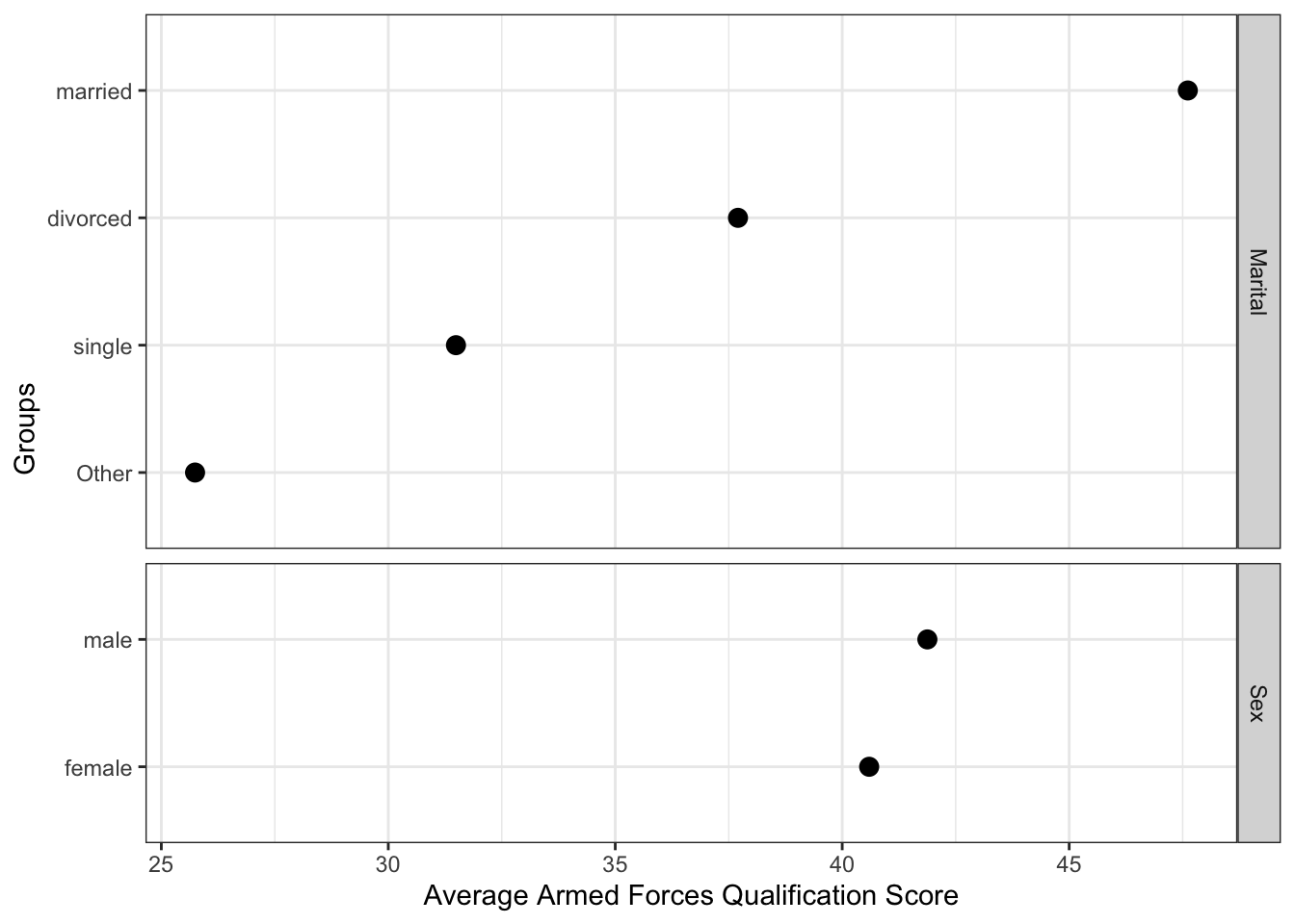
Since we computed standard errors, we could also add error bars using geom_errorbarh.
ggplot(comb_means, aes(avg_afqt, fct_reorder(levels, avg_afqt))) +
  geom_point(size = 3) +
  geom_errorbarh(aes(xmin = avg_afqt - se_mean*2, xmax = avg_afqt + se_mean*2),
                 height = 0) +
  facet_grid(group ~ ., scales = 'free', space = 'free') +
  ylab("Groups") +
  xlab("Average Armed Forces Qualification Score") +
  theme_bw()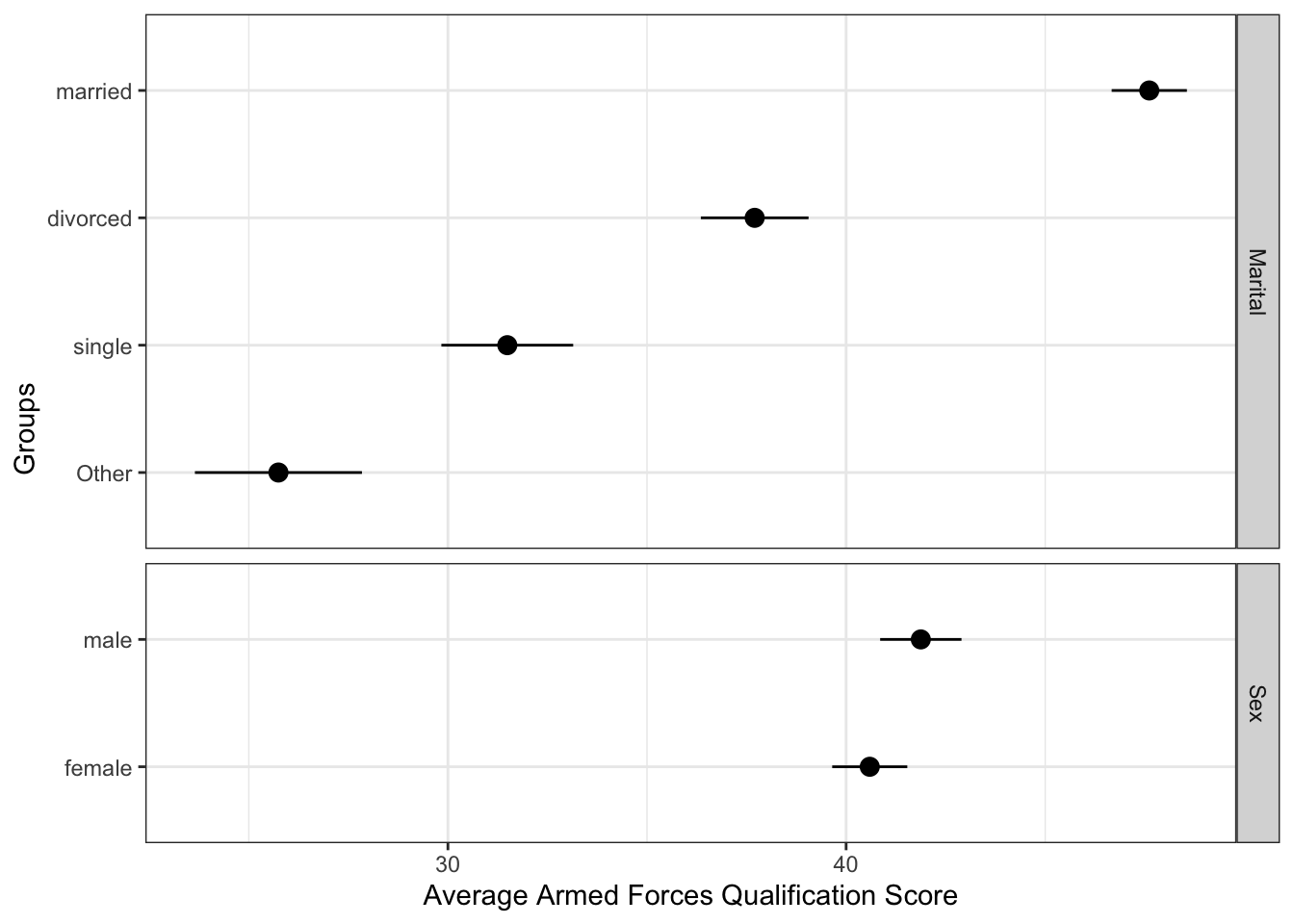
Plotting the interaction happens in a similar fashion. Namely, we will now calculate means by using both variables in a single group_by statement.
int_means <- heights %>%
  group_by(marital_comb, sex) %>%
  summarise(avg_afqt = mean(afqt, na.rm = TRUE),
            sd_afqt = sd(afqt, na.rm = TRUE),
            n = n()) %>%
  mutate(se_mean = sd_afqt/sqrt(n))
## `summarise()` has grouped output by 'marital_comb'. You can override using the
## `.groups` argument.int_means## # A tibble: 8 × 6
## # Groups: marital_comb [4]
## marital_comb sex avg_afqt sd_afqt n se_mean
## <fct> <fct> <dbl> <dbl> <int> <dbl>
## 1 single male 31.4 28.2 624 1.13
## 2 single female 31.6 27.3 500 1.22
## 3 married male 48.0 29.8 1905 0.683
## 4 married female 47.3 28.5 1901 0.653
## 5 Other male 28.8 25.7 177 1.93
## 6 Other female 24.2 23.1 350 1.24
## 7 divorced male 37.7 27.7 696 1.05
## 8 divorced female 37.7 25.7 853 0.879These means should now match the last model from the previous lecture. We can now plot these directly.
ggplot(int_means, aes(avg_afqt, fct_reorder(marital_comb, avg_afqt),
                      shape = sex, linetype = sex, group = sex)) +
  geom_point(size = 3) +
  geom_line(size = 1) +
  ylab("Groups") +
  xlab("Average Armed Forces Qualification Score") +
  theme_bw()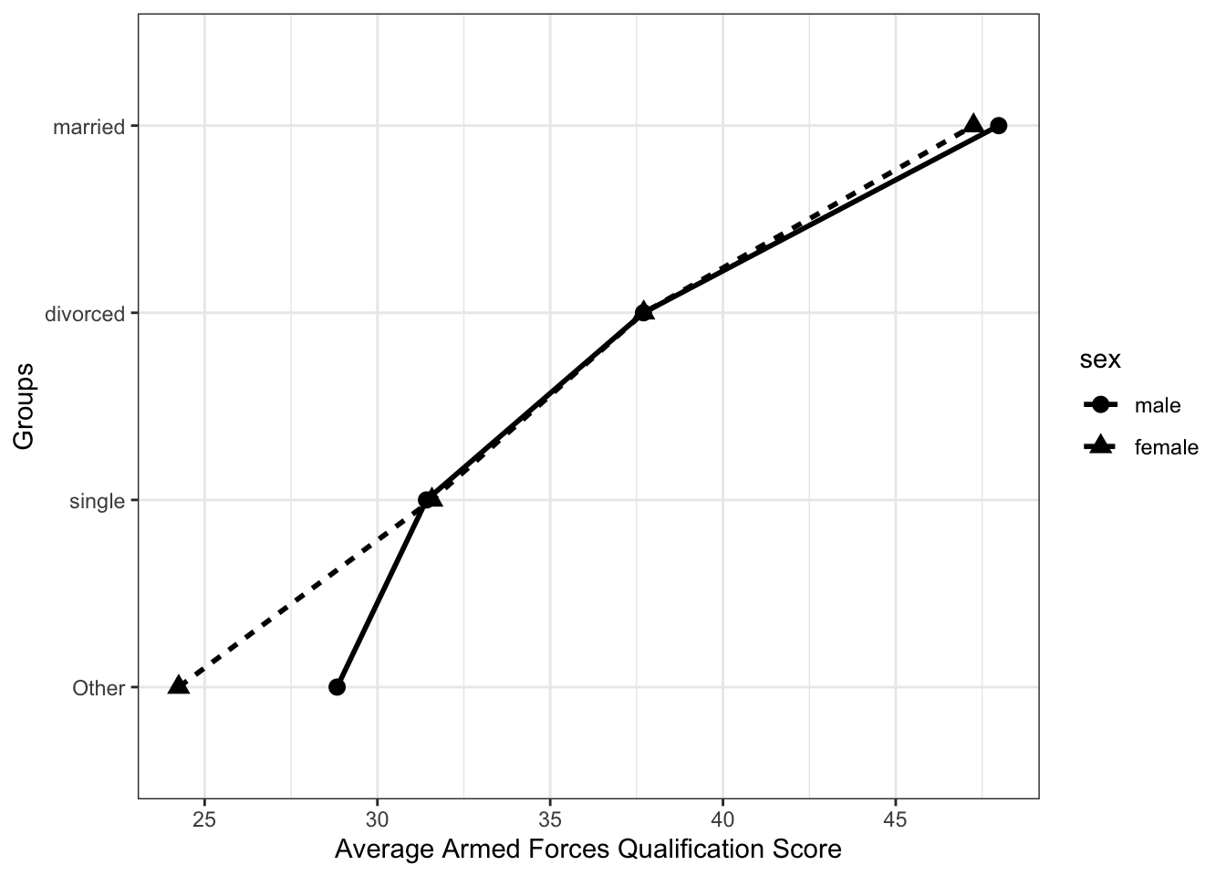
Standard error bars can be shown here, but may complicate the figure too much.
ggplot(int_means, aes(avg_afqt, fct_reorder(marital_comb, avg_afqt),
                      shape = sex, linetype = sex, group = sex)) +
  geom_point(size = 3) +
  geom_line(size = 1) +
  geom_errorbarh(aes(xmin = avg_afqt - se_mean * 2, xmax = avg_afqt + se_mean * 2),
                 height = 0) +
  ylab("Groups") +
  xlab("Average Armed Forces Qualification Score") +
  theme_bw()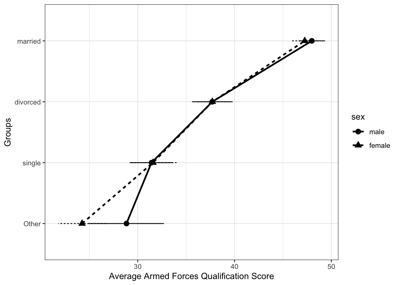
Exercises
- Using the gss_cat data from the forcats package, fit a model that predicts age with marital status, partyid, and the interaction between the two.
- Create a figure that explores the interaction between the two variables.
- Add a third variable to the model, race. Include this as a main effect, plus interacting with the other variables.
Interaction between continuous and categorical predictors
Using again the heights data, suppose we wished to again predict the Armed Forces Qualifications Test score (afqt) with marital status and height. This can be done with the linear model.
summary(lm(afqt ~ marital_comb + height, data = heights))##
## Call:
## lm(formula = afqt ~ marital_comb + height, data = heights)
##
## Residuals:
## Min 1Q Median 3Q Max
## -53.150 -22.517 -4.248 22.097 78.355
##
## Coefficients:
## Estimate Std. Error t value Pr(>|t|)
## (Intercept) -28.99932 5.67144 -5.113 3.25e-07 ***
## marital_combmarried 16.13531 0.96385 16.741 < 2e-16 ***
## marital_combOther -4.63978 1.50160 -3.090 0.00201 **
## marital_combdivorced 6.75490 1.11278 6.070 1.35e-09 ***
## height 0.89847 0.08329 10.787 < 2e-16 ***
## ---
## Signif. codes: 0 '***' 0.001 '**' 0.01 '*' 0.05 '.' 0.1 ' ' 1
##
## Residual standard error: 27.78 on 6739 degrees of freedom
## (262 observations deleted due to missingness)
## Multiple R-squared: 0.08467, Adjusted R-squared: 0.08413
## F-statistic: 155.8 on 4 and 6739 DF, p-value: < 2.2e-16You’ll notice here that the intercept is negative. Why is this negative? You can most easily see this by looking at a figure of the data. Note, here I am simply showing the dependent and the height variable ignoring the marital status, however, this will have a slightly different slope than the one above (Try it).
ggplot(heights, aes(x = height, y = afqt)) +
  geom_jitter(size = 2) +
  geom_abline(intercept = -26.02, slope = 1.002, size = 1, color = 'blue') +
  coord_cartesian(xlim = c(0, 90), ylim = c(-30, 105)) +
  ylab("Average Armed Forces Qualification Score") +
  xlab("Height") +
  theme_bw()
## Warning: Removed 262 rows containing missing values (geom_point).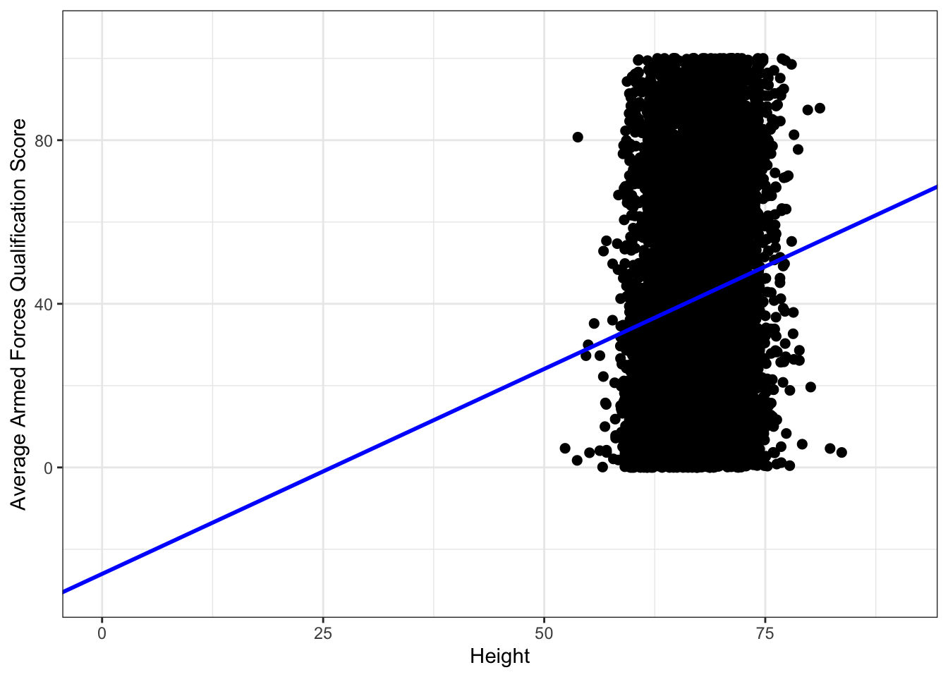
It may be better to mean center the height variable.
summary(lm(afqt ~ marital_comb + I(height - mean(heights$height)), data = heights))##
## Call:
## lm(formula = afqt ~ marital_comb + I(height - mean(heights$height)),
## data = heights)
##
## Residuals:
## Min 1Q Median 3Q Max
## -53.150 -22.517 -4.248 22.097 78.355
##
## Coefficients:
## Estimate Std. Error t value Pr(>|t|)
## (Intercept) 31.29186 0.84798 36.90 < 2e-16 ***
## marital_combmarried 16.13531 0.96385 16.74 < 2e-16 ***
## marital_combOther -4.63978 1.50160 -3.09 0.00201 **
## marital_combdivorced 6.75490 1.11278 6.07 1.35e-09 ***
## I(height - mean(heights$height)) 0.89847 0.08329 10.79 < 2e-16 ***
## ---
## Signif. codes: 0 '***' 0.001 '**' 0.01 '*' 0.05 '.' 0.1 ' ' 1
##
## Residual standard error: 27.78 on 6739 degrees of freedom
## (262 observations deleted due to missingness)
## Multiple R-squared: 0.08467, Adjusted R-squared: 0.08413
## F-statistic: 155.8 on 4 and 6739 DF, p-value: < 2.2e-16Notice that the mean effects do not change, but rather just the location of the intercept. This is a traditional analysis of covariance model.
Interactions are simple to add now, they follow the same syntax as the categorical predictors from above. For example, if we wanted to add an interaction between height and marital status, we could do this as follows.
summary(lm(afqt ~ marital_comb + I(height - mean(heights$height)) +
             marital_comb:I(height - mean(heights$height)),
           data = heights))
##
## Call:
## lm(formula = afqt ~ marital_comb + I(height - mean(heights$height)) +
## marital_comb:I(height - mean(heights$height)), data = heights)
##
## Residuals:
## Min 1Q Median 3Q Max
## -53.768 -22.664 -4.183 21.972 78.762
##
## Coefficients:
## Estimate Std. Error
## (Intercept) 31.32214 0.84911
## marital_combmarried 16.08587 0.96531
## marital_combOther -4.58940 1.53070
## marital_combdivorced 6.66304 1.11478
## I(height - mean(heights$height)) 0.76180 0.20923
## marital_combmarried:I(height - mean(heights$height)) 0.22912 0.23745
## marital_combOther:I(height - mean(heights$height)) 0.21641 0.37137
## marital_combdivorced:I(height - mean(heights$height)) -0.02469 0.27510
## t value Pr(>|t|)
## (Intercept) 36.888 < 2e-16 ***
## marital_combmarried 16.664 < 2e-16 ***
## marital_combOther -2.998 0.002725 **
## marital_combdivorced 5.977 2.39e-09 ***
## I(height - mean(heights$height)) 3.641 0.000274 ***
## marital_combmarried:I(height - mean(heights$height)) 0.965 0.334624
## marital_combOther:I(height - mean(heights$height)) 0.583 0.560092
## marital_combdivorced:I(height - mean(heights$height)) -0.090 0.928481
## ---
## Signif. codes: 0 '***' 0.001 '**' 0.01 '*' 0.05 '.' 0.1 ' ' 1
##
## Residual standard error: 27.79 on 6736 degrees of freedom
## (262 observations deleted due to missingness)
## Multiple R-squared: 0.08494, Adjusted R-squared: 0.08399
## F-statistic: 89.32 on 7 and 6736 DF, p-value: < 2.2e-16or
summary(lm(afqt ~ marital_comb * I(height - mean(heights$height)), data = heights))##
## Call:
## lm(formula = afqt ~ marital_comb * I(height - mean(heights$height)),
## data = heights)
##
## Residuals:
## Min 1Q Median 3Q Max
## -53.768 -22.664 -4.183 21.972 78.762
##
## Coefficients:
## Estimate Std. Error
## (Intercept) 31.32214 0.84911
## marital_combmarried 16.08587 0.96531
## marital_combOther -4.58940 1.53070
## marital_combdivorced 6.66304 1.11478
## I(height - mean(heights$height)) 0.76180 0.20923
## marital_combmarried:I(height - mean(heights$height)) 0.22912 0.23745
## marital_combOther:I(height - mean(heights$height)) 0.21641 0.37137
## marital_combdivorced:I(height - mean(heights$height)) -0.02469 0.27510
## t value Pr(>|t|)
## (Intercept) 36.888 < 2e-16 ***
## marital_combmarried 16.664 < 2e-16 ***
## marital_combOther -2.998 0.002725 **
## marital_combdivorced 5.977 2.39e-09 ***
## I(height - mean(heights$height)) 3.641 0.000274 ***
## marital_combmarried:I(height - mean(heights$height)) 0.965 0.334624
## marital_combOther:I(height - mean(heights$height)) 0.583 0.560092
## marital_combdivorced:I(height - mean(heights$height)) -0.090 0.928481
## ---
## Signif. codes: 0 '***' 0.001 '**' 0.01 '*' 0.05 '.' 0.1 ' ' 1
##
## Residual standard error: 27.79 on 6736 degrees of freedom
## (262 observations deleted due to missingness)
## Multiple R-squared: 0.08494, Adjusted R-squared: 0.08399
## F-statistic: 89.32 on 7 and 6736 DF, p-value: < 2.2e-16What do these coefficients mean however? This is best explained with a picture.
model_summary <- augment(lm(afqt ~ marital_comb * I(height - mean(heights$height)),
                            data = heights))
model_summary <- rename(model_summary, 'height_center' = `I(height - mean(heights$height))`)
model_summary
## # A tibble: 6,744 × 9
## .rownames afqt marital_comb height_center .fitted .hat .sigma .cooksd
## <chr> <dbl> <fct> <I<dbl>> <dbl> <dbl> <dbl> <dbl>
## 1 1 6.84 married -7.10 40.4 0.00115 27.8 2.09e-4
## 2 2 49.4 married 2.90 50.3 0.000390 27.8 4.39e-8
## 3 3 99.4 married -2.10 45.3 0.000360 27.8 1.70e-4
## 4 4 44.0 married -4.10 43.3 0.000576 27.8 4.33e-8
## 5 5 59.7 married -1.10 46.3 0.000301 27.8 8.70e-6
## 6 6 98.8 divorced 0.896 38.6 0.000737 27.8 4.33e-4
## 7 7 82.3 married 6.90 54.2 0.00100 27.8 1.28e-4
## 8 8 50.3 divorced -3.10 35.7 0.000976 27.8 3.37e-5
## 9 9 89.7 divorced 1.90 39.4 0.000884 27.8 3.63e-4
## 10 10 96.0 divorced 1.90 39.4 0.000884 27.8 4.59e-4
## # … with 6,734 more rows, and 1 more variable: .std.resid <dbl>ggplot(model_summary, aes(height_center, afqt)) +
geom_jitter(alpha = .1) +
geom_line(aes(x = height_center, y = .fitted, color = marital_comb),
size = 2) +
ylab("Average Armed Forces Qualification Score") +
xlab("Height") +
theme_bw()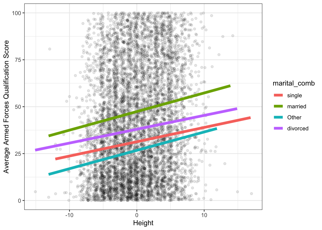
The figure for the traditional ANCOVA model initially explored would look like:
model_summary <- augment(lm(afqt ~ marital_comb + I(height - mean(heights$height)),
                            data = heights))
model_summary <- rename(model_summary, 'height_center' = `I(height - mean(heights$height))`)
model_summary
## # A tibble: 6,744 × 9
## .rownames afqt marital_comb height_center .fitted .hat .sigma .cooksd
## <chr> <dbl> <fct> <I<dbl>> <dbl> <dbl> <dbl> <dbl>
## 1 1 6.84 married -7.10 41.0 0.000753 27.8 2.29e-4
## 2 2 49.4 married 2.90 50.0 0.000337 27.8 2.99e-8
## 3 3 99.4 married -2.10 45.5 0.000320 27.8 2.41e-4
## 4 4 44.0 married -4.10 43.7 0.000439 27.8 9.09e-9
## 5 5 59.7 married -1.10 46.4 0.000288 27.8 1.31e-5
## 6 6 98.8 divorced 0.896 38.9 0.000684 27.8 6.38e-4
## 7 7 82.3 married 6.90 53.6 0.000674 27.8 1.44e-4
## 8 8 50.3 divorced -3.10 35.3 0.000736 27.8 4.31e-5
## 9 9 89.7 divorced 1.90 39.7 0.000716 27.8 4.63e-4
## 10 10 96.0 divorced 1.90 39.7 0.000716 27.8 5.88e-4
## # … with 6,734 more rows, and 1 more variable: .std.resid <dbl>ggplot(model_summary, aes(height_center, afqt)) +
geom_jitter(alpha = .1) +
geom_line(aes(x = height_center, y = .fitted, color = marital_comb),
size = 2) +
ylab("Average Armed Forces Qualification Score") +
xlab("Height") +
theme_bw()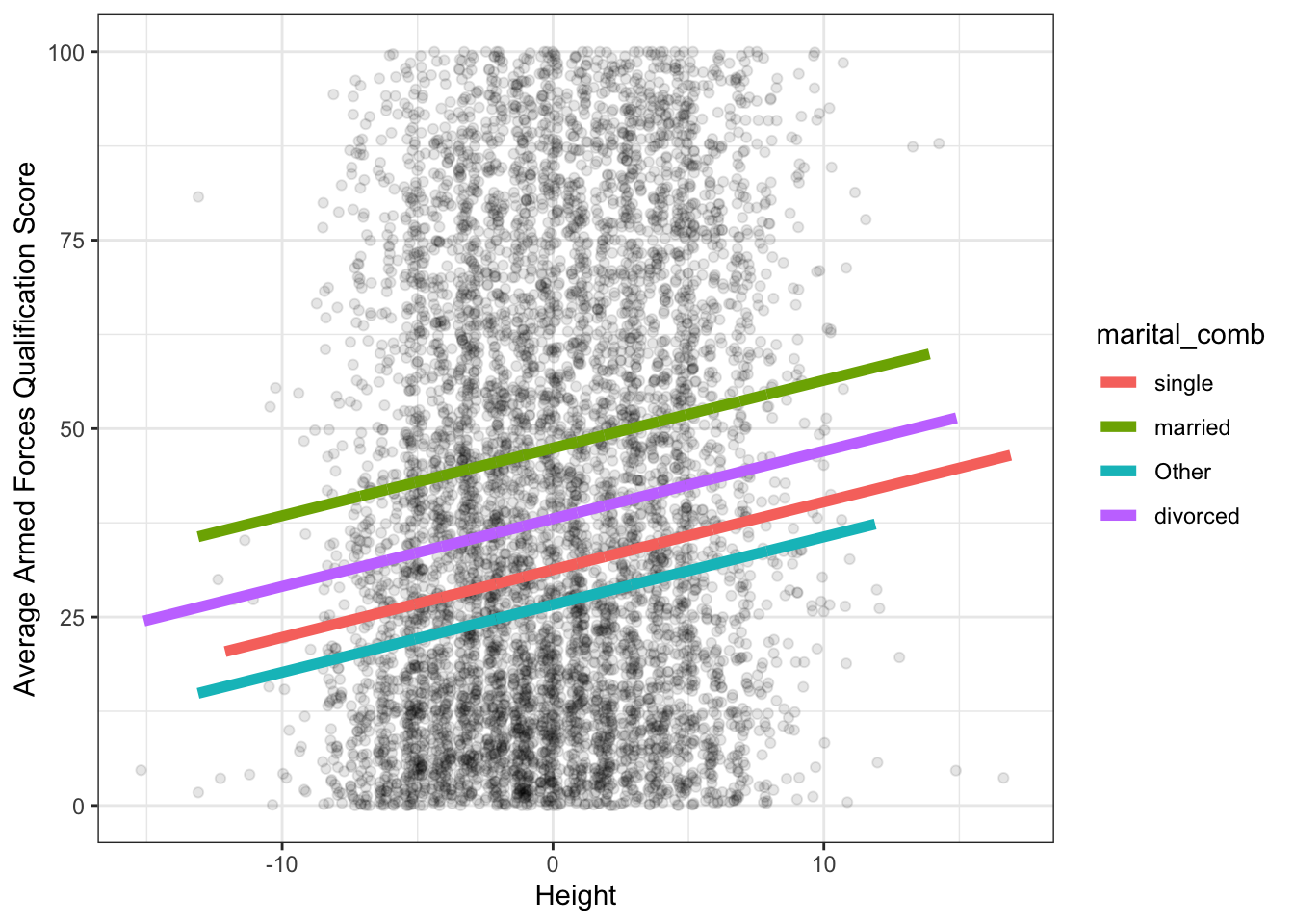
Exercises
- Using the gss_cat data from the forcats package, fit a model that predicts age with marital status, tvhours, and the interaction between the two.
- Interpret the parameter estimates from this model? Is there evidence that the interaction is adding to the model?
- Create a figure that explores the interaction between the two variables.
- Fit another model that predicts age with marital status, party affiliation, and tvhours (main effects) as well as the interaction between marital status and tvhours and party afilliation and tvhours (two second order interactions).
- Interpret the effects for this model.