Data Manipulation
Data munging (i.e. data transformations, variable creation, filtering) is a common task that is often overlooked in traditional statistics textbooks and courses. Even though it is omitted, the task of cleaning and organizing the data (coming in week 5 of the course)
Data from the fivethirtyeight package is used in this set of notes to show the use of the dplyr verbs for data munging. This package can be installed with the following command:
install.packages("fivethirtyeight")To get started with this set of notes, you will need the following packages loaded:
library(fivethirtyeight)
library(tidyverse)
We are going to explore the congress_age data set in more detail. Take a few minutes to familiarize yourself with the data.
View(congress_age)
?congress_agecongress_age## # A tibble: 18,635 × 13
## congress chamber bioguide firstname middlename lastname suffix birthday
## <int> <chr> <chr> <chr> <chr> <chr> <chr> <date>
## 1 80 house M000112 Joseph Jefferson Mansfield <NA> 1861-02-09
## 2 80 house D000448 Robert Lee Doughton <NA> 1863-11-07
## 3 80 house S000001 Adolph Joachim Sabath <NA> 1866-04-04
## 4 80 house E000023 Charles Aubrey Eaton <NA> 1868-03-29
## 5 80 house L000296 William <NA> Lewis <NA> 1868-09-22
## 6 80 house G000017 James A. Gallagher <NA> 1869-01-16
## 7 80 house W000265 Richard Joseph Welch <NA> 1869-02-13
## 8 80 house B000565 Sol <NA> Bloom <NA> 1870-03-09
## 9 80 house H000943 Merlin <NA> Hull <NA> 1870-12-18
## 10 80 house G000169 Charles Laceille Gifford <NA> 1871-03-15
## # … with 18,625 more rows, and 5 more variables: state <chr>, party <chr>,
## # incumbent <lgl>, termstart <date>, age <dbl>Using dplyr for data munging
The dplyr package uses verbs for common data manipulation tasks. These include:
filter()arrange()select()mutate()summarise()
The great aspect of these verbs are that they all take a similar data structure, the first argument is always the data, the other arguments are unquoted column names. These functions also always return a data frame in which the rows are observations and the columns are variables.
Examples with filter()
The filter function selects rows that match a specified condition(s). For example, suppose we wanted to select only the rows in the data that are a part of the 80th congress. The following code will do this action:
filter(congress_age, congress == 80)## # A tibble: 555 × 13
## congress chamber bioguide firstname middlename lastname suffix birthday
## <int> <chr> <chr> <chr> <chr> <chr> <chr> <date>
## 1 80 house M000112 Joseph Jefferson Mansfield <NA> 1861-02-09
## 2 80 house D000448 Robert Lee Doughton <NA> 1863-11-07
## 3 80 house S000001 Adolph Joachim Sabath <NA> 1866-04-04
## 4 80 house E000023 Charles Aubrey Eaton <NA> 1868-03-29
## 5 80 house L000296 William <NA> Lewis <NA> 1868-09-22
## 6 80 house G000017 James A. Gallagher <NA> 1869-01-16
## 7 80 house W000265 Richard Joseph Welch <NA> 1869-02-13
## 8 80 house B000565 Sol <NA> Bloom <NA> 1870-03-09
## 9 80 house H000943 Merlin <NA> Hull <NA> 1870-12-18
## 10 80 house G000169 Charles Laceille Gifford <NA> 1871-03-15
## # … with 545 more rows, and 5 more variables: state <chr>, party <chr>,
## # incumbent <lgl>, termstart <date>, age <dbl>Notice from above two things, first, the function returned a new data frame. Therefore, if this subsetted data is to be saved, we need to save it to an object, for example, as follows:
congress_80 <- filter(congress_age, congress == 80)Notice now that the data were not automatically printed, instead it was saved into the object called congress_80. If you wish to preview the data and save it to an object in a single step, you need to wrap the command above in parentheses. Take a second to try this yourself.
Secondly, notice from the above commands that equality in R is done with == not just a single =. The single = is used for named arguments, therefore when testing for equality you need to be sure to use ==, this is a common frustration and source of bugs when getting started with R.
Selecting values based on a character vector are similar to numeric values. For example, suppose we wanted to select only those rows pertaining to those from the senate. The following code will do that:
senate <- filter(congress_age, chamber == 'senate')Combining Logical Operations
The filter function becomes much more useful with more complex operations. For example, suppose we were interested in selecting the rows that belong to the 80th senate.
filter(congress_age, congress == 80, chamber == 'senate')## # A tibble: 102 × 13
## congress chamber bioguide firstname middlename lastname suffix birthday
## <int> <chr> <chr> <chr> <chr> <chr> <chr> <date>
## 1 80 senate C000133 Arthur <NA> Capper <NA> 1865-07-14
## 2 80 senate G000418 Theodore Francis Green <NA> 1867-10-02
## 3 80 senate M000499 Kenneth Douglas McKellar <NA> 1869-01-29
## 4 80 senate R000112 Clyde Martin Reed <NA> 1871-10-19
## 5 80 senate M000895 Edward Hall Moore <NA> 1871-11-19
## 6 80 senate O000146 John Holmes Overton <NA> 1875-09-17
## 7 80 senate M001108 James Edward Murray <NA> 1876-05-03
## 8 80 senate M000308 Patrick Anthony McCarran <NA> 1876-08-08
## 9 80 senate T000165 Elmer <NA> Thomas <NA> 1876-09-08
## 10 80 senate W000021 Robert Ferdinand Wagner <NA> 1877-06-08
## # … with 92 more rows, and 5 more variables: state <chr>, party <chr>,
## # incumbent <lgl>, termstart <date>, age <dbl>By default, the filter function uses AND when combining multiple arguments. Therefore, the above command returned only the 102 rows belonging to senators from the 80th congress. The figure on section 5.2.2 of R for Data Science shows all the possible boolean operators.
Using an example of the OR operator using | to select the 80th and 81st congress:
filter(congress_age, congress == 80 | congress == 81)## # A tibble: 1,112 × 13
## congress chamber bioguide firstname middlename lastname suffix birthday
## <int> <chr> <chr> <chr> <chr> <chr> <chr> <date>
## 1 80 house M000112 Joseph Jefferson Mansfield <NA> 1861-02-09
## 2 80 house D000448 Robert Lee Doughton <NA> 1863-11-07
## 3 80 house S000001 Adolph Joachim Sabath <NA> 1866-04-04
## 4 80 house E000023 Charles Aubrey Eaton <NA> 1868-03-29
## 5 80 house L000296 William <NA> Lewis <NA> 1868-09-22
## 6 80 house G000017 James A. Gallagher <NA> 1869-01-16
## 7 80 house W000265 Richard Joseph Welch <NA> 1869-02-13
## 8 80 house B000565 Sol <NA> Bloom <NA> 1870-03-09
## 9 80 house H000943 Merlin <NA> Hull <NA> 1870-12-18
## 10 80 house G000169 Charles Laceille Gifford <NA> 1871-03-15
## # … with 1,102 more rows, and 5 more variables: state <chr>, party <chr>,
## # incumbent <lgl>, termstart <date>, age <dbl>Note that to do the OR operator, you need to name the variable twice. When selecting multiple values in the same variable, a handy shortcut is %in%. The same command can be run with the following shorthand: handy shortcut is %in%. The same command can be run with the following shorthard
filter(congress_age, congress %in% c(80, 81))## # A tibble: 1,112 × 13
## congress chamber bioguide firstname middlename lastname suffix birthday
## <int> <chr> <chr> <chr> <chr> <chr> <chr> <date>
## 1 80 house M000112 Joseph Jefferson Mansfield <NA> 1861-02-09
## 2 80 house D000448 Robert Lee Doughton <NA> 1863-11-07
## 3 80 house S000001 Adolph Joachim Sabath <NA> 1866-04-04
## 4 80 house E000023 Charles Aubrey Eaton <NA> 1868-03-29
## 5 80 house L000296 William <NA> Lewis <NA> 1868-09-22
## 6 80 house G000017 James A. Gallagher <NA> 1869-01-16
## 7 80 house W000265 Richard Joseph Welch <NA> 1869-02-13
## 8 80 house B000565 Sol <NA> Bloom <NA> 1870-03-09
## 9 80 house H000943 Merlin <NA> Hull <NA> 1870-12-18
## 10 80 house G000169 Charles Laceille Gifford <NA> 1871-03-15
## # … with 1,102 more rows, and 5 more variables: state <chr>, party <chr>,
## # incumbent <lgl>, termstart <date>, age <dbl>Not Operator
Another useful operator that deserves a bit more discussion is the not operator, !. For example, suppose we wanted to omit the 80th congress:
filter(congress_age, congress != 80)## # A tibble: 18,080 × 13
## congress chamber bioguide firstname middlename lastname suffix birthday
## <int> <chr> <chr> <chr> <chr> <chr> <chr> <date>
## 1 81 house D000448 Robert Lee Doughton <NA> 1863-11-07
## 2 81 house S000001 Adolph Joachim Sabath <NA> 1866-04-04
## 3 81 house E000023 Charles Aubrey Eaton <NA> 1868-03-29
## 4 81 house W000265 Richard Joseph Welch <NA> 1869-02-13
## 5 81 house B000565 Sol <NA> Bloom <NA> 1870-03-09
## 6 81 house H000943 Merlin <NA> Hull <NA> 1870-12-18
## 7 81 house B000545 Schuyler Otis Bland <NA> 1872-05-04
## 8 81 house K000138 John Hosea Kerr <NA> 1873-12-31
## 9 81 house C000932 Robert <NA> Crosser <NA> 1874-06-07
## 10 81 house K000039 John <NA> Kee <NA> 1874-08-22
## # … with 18,070 more rows, and 5 more variables: state <chr>, party <chr>,
## # incumbent <lgl>, termstart <date>, age <dbl>It is also possible to do not with an AND operator as follows:
filter(congress_age, congress == 80 & !chamber == 'senate')## # A tibble: 453 × 13
## congress chamber bioguide firstname middlename lastname suffix birthday
## <int> <chr> <chr> <chr> <chr> <chr> <chr> <date>
## 1 80 house M000112 Joseph Jefferson Mansfield <NA> 1861-02-09
## 2 80 house D000448 Robert Lee Doughton <NA> 1863-11-07
## 3 80 house S000001 Adolph Joachim Sabath <NA> 1866-04-04
## 4 80 house E000023 Charles Aubrey Eaton <NA> 1868-03-29
## 5 80 house L000296 William <NA> Lewis <NA> 1868-09-22
## 6 80 house G000017 James A. Gallagher <NA> 1869-01-16
## 7 80 house W000265 Richard Joseph Welch <NA> 1869-02-13
## 8 80 house B000565 Sol <NA> Bloom <NA> 1870-03-09
## 9 80 house H000943 Merlin <NA> Hull <NA> 1870-12-18
## 10 80 house G000169 Charles Laceille Gifford <NA> 1871-03-15
## # … with 443 more rows, and 5 more variables: state <chr>, party <chr>,
## # incumbent <lgl>, termstart <date>, age <dbl>Exercises
- Using the congress data, select the rows belonging to the democrats (party = D) from the senate of the 100th congress.
- Select all congress members who are older than 80 years old.
Note on Missing Data
Missing data within R are represented with NA which stands for not available.
There are no missing data in the congress data, however, by default the filter function will not return any missing values. In order to select missing data, you need to use the is.na function.
Exercise
- Given the following simple vector, run one filter that selects all values greater than 100. Write a second filter command that selects all the rows greater than 100 and also the NA value.
df <- tibble(x = c(200, 30, NA, 45, 212))Examples with arrange()
The arrange function is used for ordering rows in the data. For example, suppose we wanted to order the rows in the congress data by the state the members of congress lived in. This can be done using the arrange function as follows:
arrange(congress_age, state)## # A tibble: 18,635 × 13
## congress chamber bioguide firstname middlename lastname suffix birthday
## <int> <chr> <chr> <chr> <chr> <chr> <chr> <date>
## 1 80 house B000201 Edward Lewis Bartlett <NA> 1904-04-20
## 2 81 house B000201 Edward Lewis Bartlett <NA> 1904-04-20
## 3 82 house B000201 Edward Lewis Bartlett <NA> 1904-04-20
## 4 83 house B000201 Edward Lewis Bartlett <NA> 1904-04-20
## 5 84 house B000201 Edward Lewis Bartlett <NA> 1904-04-20
## 6 85 house B000201 Edward Lewis Bartlett <NA> 1904-04-20
## 7 86 house R000282 Ralph Julian Rivers <NA> 1903-05-23
## 8 86 senate G000508 Ernest <NA> Gruening <NA> 1887-02-06
## 9 86 senate B000201 Edward Lewis Bartlett <NA> 1904-04-20
## 10 87 house R000282 Ralph Julian Rivers <NA> 1903-05-23
## # … with 18,625 more rows, and 5 more variables: state <chr>, party <chr>,
## # incumbent <lgl>, termstart <date>, age <dbl>Similar to the filter function, additional arguments can be added to add more layers to the ordering. For example, if we were interested in ordering the rows by state and then by party affiliation.
arrange(congress_age, state, party)## # A tibble: 18,635 × 13
## congress chamber bioguide firstname middlename lastname suffix birthday
## <int> <chr> <chr> <chr> <chr> <chr> <chr> <date>
## 1 80 house B000201 Edward Lewis Bartlett <NA> 1904-04-20
## 2 81 house B000201 Edward Lewis Bartlett <NA> 1904-04-20
## 3 82 house B000201 Edward Lewis Bartlett <NA> 1904-04-20
## 4 83 house B000201 Edward Lewis Bartlett <NA> 1904-04-20
## 5 84 house B000201 Edward Lewis Bartlett <NA> 1904-04-20
## 6 85 house B000201 Edward Lewis Bartlett <NA> 1904-04-20
## 7 86 house R000282 Ralph Julian Rivers <NA> 1903-05-23
## 8 86 senate G000508 Ernest <NA> Gruening <NA> 1887-02-06
## 9 86 senate B000201 Edward Lewis Bartlett <NA> 1904-04-20
## 10 87 house R000282 Ralph Julian Rivers <NA> 1903-05-23
## # … with 18,625 more rows, and 5 more variables: state <chr>, party <chr>,
## # incumbent <lgl>, termstart <date>, age <dbl>More variables can easily be added to the arrange function. Notice from the above two commands that the ordering of the rows is in ascending order, if descending order is desired, the desc function. For example, to order the data starting with the latest congress first:
arrange(congress_age, desc(congress))## # A tibble: 18,635 × 13
## congress chamber bioguide firstname middlename lastname suffix birthday
## <int> <chr> <chr> <chr> <chr> <chr> <chr> <date>
## 1 113 house H000067 Ralph M. Hall <NA> 1923-05-03
## 2 113 house D000355 John D. Dingell <NA> 1926-07-08
## 3 113 house C000714 John <NA> Conyers Jr. 1929-05-16
## 4 113 house S000480 Louise McIntosh Slaughter <NA> 1929-08-14
## 5 113 house R000053 Charles B. Rangel <NA> 1930-06-11
## 6 113 house J000174 Sam Robert Johnson <NA> 1930-10-11
## 7 113 house Y000031 C. W. Bill Young <NA> 1930-12-16
## 8 113 house C000556 Howard <NA> Coble <NA> 1931-03-18
## 9 113 house L000263 Sander M. Levin <NA> 1931-09-06
## 10 113 house Y000033 Don E. Young <NA> 1933-06-09
## # … with 18,625 more rows, and 5 more variables: state <chr>, party <chr>,
## # incumbent <lgl>, termstart <date>, age <dbl>Examples with select()
The select function is used to select columns (i.e. variables) from the data but keep all the rows. For example, maybe we only needed the congress number, the chamber, the party affiliation, and the age of the members of congress. We can reduce the data to just these variables using select.
select(congress_age, congress, chamber, party, age)## # A tibble: 18,635 × 4
## congress chamber party age
## <int> <chr> <chr> <dbl>
## 1 80 house D 85.9
## 2 80 house D 83.2
## 3 80 house D 80.7
## 4 80 house R 78.8
## 5 80 house R 78.3
## 6 80 house R 78
## 7 80 house R 77.9
## 8 80 house D 76.8
## 9 80 house R 76
## 10 80 house R 75.8
## # … with 18,625 more rowsSimilar to the arrange functions, the variables that you wish to keep are separated by commas and come after the data argument.
For more complex selection, the dplyr package has additional functions that are helpful for variable selection. These include:
- starts_with()
- ends_with()
- contains()
- matches()
- num_range()
These helper functions can be useful for selecting many variables that match a specific pattern. For example, suppose we were interested in selecting all the name variables, this can be accomplished using the contains function as follows:
select(congress_age, contains('name'))## # A tibble: 18,635 × 3
## firstname middlename lastname
## <chr> <chr> <chr>
## 1 Joseph Jefferson Mansfield
## 2 Robert Lee Doughton
## 3 Adolph Joachim Sabath
## 4 Charles Aubrey Eaton
## 5 William <NA> Lewis
## 6 James A. Gallagher
## 7 Richard Joseph Welch
## 8 Sol <NA> Bloom
## 9 Merlin <NA> Hull
## 10 Charles Laceille Gifford
## # … with 18,625 more rowsAnother useful shorthand to select multiple columns in succession is the : operator. For example, suppose we wanted to select all the variables between congress and bithday.
select(congress_age, congress:birthday)## # A tibble: 18,635 × 8
## congress chamber bioguide firstname middlename lastname suffix birthday
## <int> <chr> <chr> <chr> <chr> <chr> <chr> <date>
## 1 80 house M000112 Joseph Jefferson Mansfield <NA> 1861-02-09
## 2 80 house D000448 Robert Lee Doughton <NA> 1863-11-07
## 3 80 house S000001 Adolph Joachim Sabath <NA> 1866-04-04
## 4 80 house E000023 Charles Aubrey Eaton <NA> 1868-03-29
## 5 80 house L000296 William <NA> Lewis <NA> 1868-09-22
## 6 80 house G000017 James A. Gallagher <NA> 1869-01-16
## 7 80 house W000265 Richard Joseph Welch <NA> 1869-02-13
## 8 80 house B000565 Sol <NA> Bloom <NA> 1870-03-09
## 9 80 house H000943 Merlin <NA> Hull <NA> 1870-12-18
## 10 80 house G000169 Charles Laceille Gifford <NA> 1871-03-15
## # … with 18,625 more rowsRename variables
The select function does allow you to rename variables, however, using the select function to rename variables is not usually advised as you may end up missing a variable that you wish to keep during the renaming operation. Instead, using the rename function is better practice.
rename(congress_age, first_name = firstname, last_name = lastname)## # A tibble: 18,635 × 13
## congress chamber bioguide first_name middlename last_name suffix birthday
## <int> <chr> <chr> <chr> <chr> <chr> <chr> <date>
## 1 80 house M000112 Joseph Jefferson Mansfield <NA> 1861-02-09
## 2 80 house D000448 Robert Lee Doughton <NA> 1863-11-07
## 3 80 house S000001 Adolph Joachim Sabath <NA> 1866-04-04
## 4 80 house E000023 Charles Aubrey Eaton <NA> 1868-03-29
## 5 80 house L000296 William <NA> Lewis <NA> 1868-09-22
## 6 80 house G000017 James A. Gallagher <NA> 1869-01-16
## 7 80 house W000265 Richard Joseph Welch <NA> 1869-02-13
## 8 80 house B000565 Sol <NA> Bloom <NA> 1870-03-09
## 9 80 house H000943 Merlin <NA> Hull <NA> 1870-12-18
## 10 80 house G000169 Charles Laceille Gifford <NA> 1871-03-15
## # … with 18,625 more rows, and 5 more variables: state <chr>, party <chr>,
## # incumbent <lgl>, termstart <date>, age <dbl>By default, the rename function will not save changes to the object, if you wish to save the name differences (very likely), be sure to save this new step to an object.
Exercises
- Using the
dplyrhelper functions, select all the variables that start with the letter ‘c’. - Rename the first three variables in the congress data to ‘x1’, ‘x2’, ‘x3’.
- After renaming the first three variables, use this new data (ensure you saved the previous step to an object) to select these three variables with the
num_rangefunction.
Examples with mutate()
mutate is a useful verb that allows you to add new columns to the existing data set. Actions done with mutate include adding a column of means, counts, or other transformations of existing variables. Suppose for example, we wished to convert the party affiliation of the members of congress into a dummy (indicator) variable. This may be useful to more easily compute a proportion or count for instance.
This can be done with the mutate function. Below, I’m first going to use select to reduce the number of columns to make it easier to see the operation.
congress_red <- select(congress_age, congress, chamber, state, party)

mutate(congress_red,
       democrat = ifelse(party == 'D', 1, 0),
       num_democrat = sum(democrat)
       )
## # A tibble: 18,635 × 6
## congress chamber state party democrat num_democrat
## <int> <chr> <chr> <chr> <dbl> <dbl>
## 1 80 house TX D 1 10290
## 2 80 house NC D 1 10290
## 3 80 house IL D 1 10290
## 4 80 house NJ R 0 10290
## 5 80 house KY R 0 10290
## 6 80 house PA R 0 10290
## 7 80 house CA R 0 10290
## 8 80 house NY D 1 10290
## 9 80 house WI R 0 10290
## 10 80 house MA R 0 10290
## # … with 18,625 more rowsYou’ll notice that the number of rows in the data are the same (18635) as it was previously, but now the two new columns have been added to the data. One converted the party affiliation to a series of 0/1 values and the other variable counted up the number of democrats elected since the 80th congress. Notice how this last variable is simply repeated for all values in the data. The operation done here is not too exciting, however, we will learn another utility later that allows us to group the data to calculate different values for each group.
Lastly, from the output above, notice that I was able to reference a variable that I created previously in the mutate command. This is unique to the dplyr package and allows you to create a single mutate command to add many variables, even those that depend on prior calculations. Obviously, if you need to reference a calculation in another calculation, they need to be done in the proper order.
Creation Functions
There are many useful operators to use when creating additional variables. The R for Data Science text has many examples shown in section 5.5.1. In general useful operators include addition, subtraction, multiplication, division, descriptive statistics (we will talk more about these in week 4), ranks, logical comparisons, and many more. The exercises will have you explore some of these operations in more detail.
Exercises
- Using the
diamondsdata, use?diamondsfor more information on the data, use themutatefunction to calculate the price per carat. Hint, this operation would involve standardizing the price variable so that all are comparable at 1 carat. - Calculate the rank of the original price variable and the new price variable calculated above using the
min_rankfunction. Are there differences in the ranking of the prices? Hint, it may be useful to test if the two ranks are equal to explore this.
Examples with summarise()
summarise is very similar to the mutate function, except instead of adding additional columns to the data, it collapses data down to a single row. For instance, doing the same operation as the example with mutate above:
congress_2 <- mutate(congress_age,
       democrat = ifelse(party == 'D', 1, 0)
       )

summarise(congress_2,
          num_democrat = sum(democrat)
          )
## # A tibble: 1 × 1
## num_democrat
## <dbl>
## 1 10290Notice now, instead of repeating the same value for all the rows as with mutate, summarise collapsed the data into a single numeric summary. Normally this is not a very interesting data activity, however, used in tandem with another function, group_by, interesting summary statistics can be calculated.
Suppose we were interested in calculating the number of democrats in each congress. This can be achieved with similar code to above, but first by grouping the data as follows:
congress_grp <- group_by(congress_2, congress)

summarise(congress_grp,
          num_democrat = sum(democrat),
          total = n(),
          prop_democrat = num_democrat / total
)
## # A tibble: 34 × 4
## congress num_democrat total prop_democrat
## <int> <dbl> <int> <dbl>
## 1 80 247 555 0.445
## 2 81 330 557 0.592
## 3 82 292 555 0.526
## 4 83 274 557 0.492
## 5 84 288 544 0.529
## 6 85 295 547 0.539
## 7 86 356 554 0.643
## 8 87 339 559 0.606
## 9 88 332 552 0.601
## 10 89 371 548 0.677
## # … with 24 more rowsNotice above, the use of the group_by function to group the data first by congress. Then this new grouped data is passed to the summarise command. As you can see from the output, the operations performed with the summarise function are done for each unique level of the congress variable. You could now easily plot these to see the trend in proportion of democrats has changed over time.
library(ggplot2)
num_dem <- summarise(congress_grp,
                     num_democrat = sum(democrat),
                     total = n(),
                     prop_democrat = num_democrat / total
)
ggplot(num_dem, aes(x = congress, y = prop_democrat)) +
  geom_line()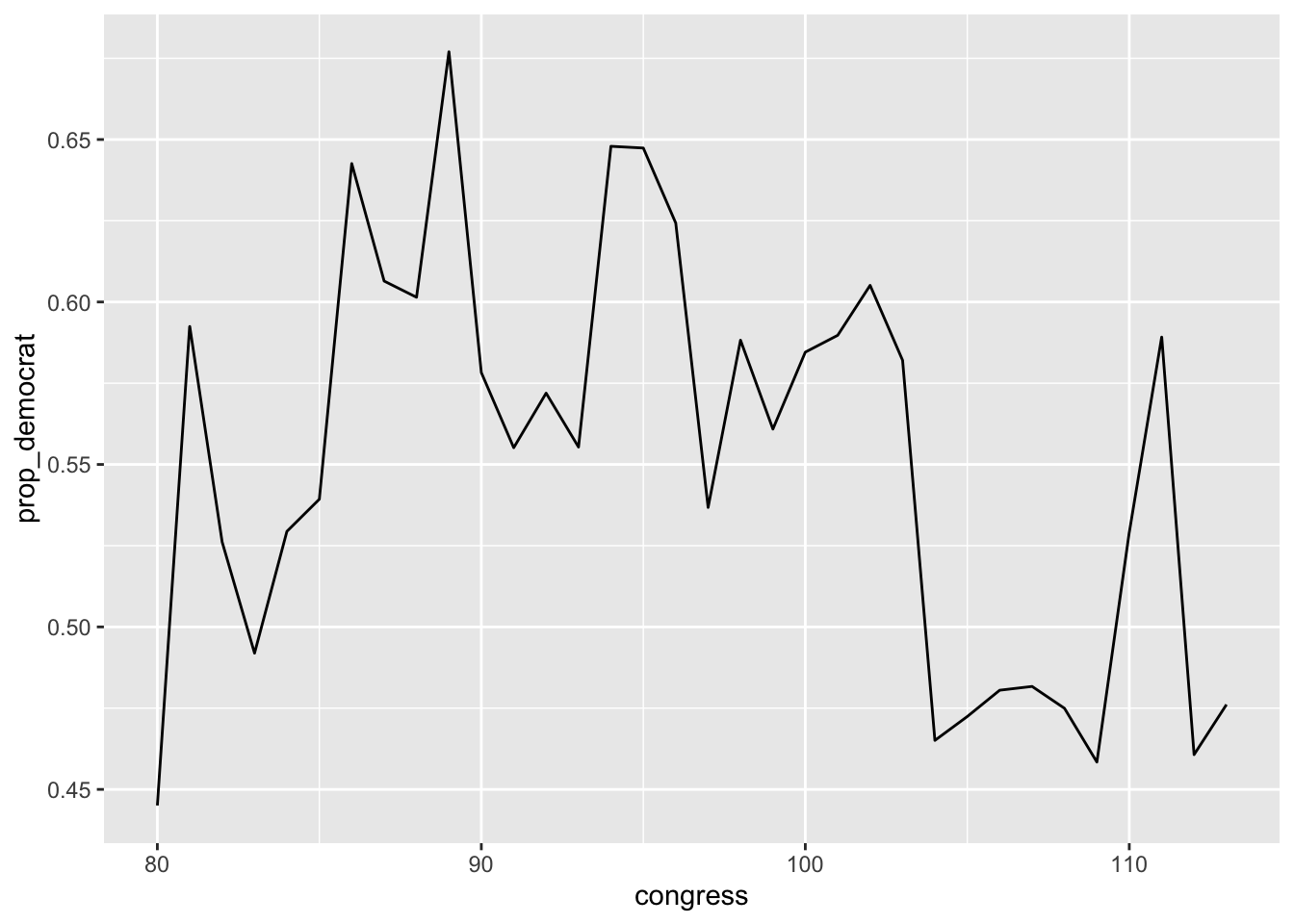
Exercises
- Suppose we wanted to calculate the number and proportion of republicans instead of democrats, assuming these are the only two parties, edit the
summarisecommand above to calculate these values. - Suppose instead of using
sum(democrat)above, we usedmean(democrat), what does this value return? Why does it return this value?
Extending group_by() in other places
The group_by function is also useful with the mutate function and works in a similar way as summarise above. For example, if we wanted to keep the values calculated above in the original data, we could use mutate instead of summarise. This would look like the following:
mutate(congress_grp,
       num_democrat = sum(democrat),
       total = n(),
       prop_democrat = num_democrat / total
)
## # A tibble: 18,635 × 17
## # Groups: congress [34]
## congress chamber bioguide firstname middlename lastname suffix birthday
## <int> <chr> <chr> <chr> <chr> <chr> <chr> <date>
## 1 80 house M000112 Joseph Jefferson Mansfield <NA> 1861-02-09
## 2 80 house D000448 Robert Lee Doughton <NA> 1863-11-07
## 3 80 house S000001 Adolph Joachim Sabath <NA> 1866-04-04
## 4 80 house E000023 Charles Aubrey Eaton <NA> 1868-03-29
## 5 80 house L000296 William <NA> Lewis <NA> 1868-09-22
## 6 80 house G000017 James A. Gallagher <NA> 1869-01-16
## 7 80 house W000265 Richard Joseph Welch <NA> 1869-02-13
## 8 80 house B000565 Sol <NA> Bloom <NA> 1870-03-09
## 9 80 house H000943 Merlin <NA> Hull <NA> 1870-12-18
## 10 80 house G000169 Charles Laceille Gifford <NA> 1871-03-15
## # … with 18,625 more rows, and 9 more variables: state <chr>, party <chr>,
## # incumbent <lgl>, termstart <date>, age <dbl>, democrat <dbl>,
## # num_democrat <dbl>, total <int>, prop_democrat <dbl>Useful summary functions
There are many useful summary functions, many of which we will explore in more detail in week 4 of the course during exploratory data analysis (EDA). However, I want to show a few here with the summarise function to ease you in. Suppose for instance we were interested in the knowing the youngest and oldest member of congress for each congress. There are actually two ways of doing this, one is using the min and max functions on the grouped data.
summarise(congress_grp,
          youngest = min(age),
          oldest = max(age)
)
## # A tibble: 34 × 3
## congress youngest oldest
## <int> <dbl> <dbl>
## 1 80 25.9 85.9
## 2 81 27.2 85.2
## 3 82 27.9 87.2
## 4 83 26.7 85.3
## 5 84 28.5 87.3
## 6 85 30.5 89.3
## 7 86 31 91.3
## 8 87 28.9 86
## 9 88 29 85.3
## 10 89 25 87.3
## # … with 24 more rowsThis could also be done by using the first and last functions after arranging the data:
summarise(arrange(congress_grp, age),
          youngest = first(age),
          oldest = last(age)
)
## # A tibble: 34 × 3
## congress youngest oldest
## <int> <dbl> <dbl>
## 1 80 25.9 85.9
## 2 81 27.2 85.2
## 3 82 27.9 87.2
## 4 83 26.7 85.3
## 5 84 28.5 87.3
## 6 85 30.5 89.3
## 7 86 31 91.3
## 8 87 28.9 86
## 9 88 29 85.3
## 10 89 25 87.3
## # … with 24 more rowsThis goes to show that there are commonly many different ways to calculate descriptive statistics. I would argue two strong virtues when writing code is to make it as clear, expressive, and ensure accuracy. Speed and grace in writing code can come later.
Exercises
- For each congress, calculate a summary using the following command:
n_distinct(state). What does this value return? - What happens when you use a logical expression within a
sumfunction call? For example, what do you get in a summarise when you do:sum(age > 75)? - What happens when you try to use
sumormeanon the variable incumbent?
Chaining together multiple operations
Now that you have seen all of the basic dplyr data manipulation verbs, it is useful to chain these together to create more complex operations. So far, I have shown you how to do it by saving intermediate steps, for example, saving the grouped data after using the group_by function. In many instances, these intermediate steps are not useful to us. In these cases you can chain operations together.
Suppose we are interested in calculating the proportion of democrats for each chamber of congress, but only since the 100th congress? There are two ways to do this, the difficult to read and the easier to read. I first shown the difficult to read.
summarise(
  group_by(
    mutate(
      filter(
        congress_age, congress >= 100
      ),
      democrat = ifelse(party == 'D', 1, 0)
    ),
    congress, chamber
  ),
  num_democrat = sum(democrat),
  total = n(),
  prop_democrat = num_democrat / total
)
## `summarise()` has grouped output by 'congress'. You can override using the
## `.groups` argument.## # A tibble: 28 × 5
## # Groups: congress [14]
## congress chamber num_democrat total prop_democrat
## <int> <chr> <dbl> <int> <dbl>
## 1 100 house 263 443 0.594
## 2 100 senate 55 101 0.545
## 3 101 house 266 445 0.598
## 4 101 senate 56 101 0.554
## 5 102 house 272 443 0.614
## 6 102 senate 59 104 0.567
## 7 103 house 261 443 0.589
## 8 103 senate 58 105 0.552
## 9 104 house 206 441 0.467
## 10 104 senate 47 103 0.456
## # … with 18 more rowsHow difficult do you find the code above to read? This is valid R code, but the first operation done is nested in the middle (it is the filter function that is run first). This makes for difficult code to debug and write in my opinion. In my opinion, the better way to write code is through the pipe operator, %>%. The same code above can be achieved with the following much easier to read code:
congress_age %>%
  filter(congress >= 100) %>%
  mutate(democrat = ifelse(party == 'D', 1, 0)) %>%
  group_by(congress, chamber) %>%
  summarise(
    num_democrat = sum(democrat),
    total = n(),
    prop_democrat = num_democrat / total
  )
## `summarise()` has grouped output by 'congress'. You can override using the
## `.groups` argument.## # A tibble: 28 × 5
## # Groups: congress [14]
## congress chamber num_democrat total prop_democrat
## <int> <chr> <dbl> <int> <dbl>
## 1 100 house 263 443 0.594
## 2 100 senate 55 101 0.545
## 3 101 house 266 445 0.598
## 4 101 senate 56 101 0.554
## 5 102 house 272 443 0.614
## 6 102 senate 59 104 0.567
## 7 103 house 261 443 0.589
## 8 103 senate 58 105 0.552
## 9 104 house 206 441 0.467
## 10 104 senate 47 103 0.456
## # … with 18 more rowsThe pipe allows for more readable code by humans and progresses from top to bottom, left to right. The best word to substitute when translating the %>% code above is ‘then’. So the code above says, using the congress_age data, then filter, then mutate, then group_by, then summarise.
This is much easier to read and follow the chain of commands. I highly recommend using the pipe in your code. For more details on what is actually happening, the R for Data Science book has a good explanation in Section 5.6.1.
Exercises
- Look at the following nested code and determine what is being done. Then translate this code to use the pipe operator.
summarise(
  group_by(
    mutate(
      filter(
        diamonds,
        color %in% c('D', 'E', 'F') & cut %in% c('Fair', 'Good', 'Very Good')
      ),
      f_color = ifelse(color == 'F', 1, 0),
      vg_cut = ifelse(cut == 'Very Good', 1, 0)
    ),
    clarity
  ),
  avg = mean(carat),
  sd = sd(carat),
  avg_p = mean(price),
  num = n(),
  summary_f_color = mean(f_color),
  summary_vg_cut = mean(vg_cut)
)