Factors
To date I have ignored factor variables and how these are implemented in R. Much of this is due to the greater flexibility of character vectors instead of factors. Also, if using the readr or readxl packages to read in data, the variables are also read in as character strings instead of factors. However, there are situations when factors are useful. Most of these uses are for readability when creating output formats for a report or paper.
This set of notes will make use of the following three packages:
library(tidyverse)
library(forcats)
library(fivethirtyeight)
Uses for Factors
To see a few of the benefits of a factor, assume we have a variable that represents the levels of a survey question with five possible responses and we only saw three of those response categories.
resp <- c('Disagree', 'Agree', 'Neutral')This type of variable has a natural order, namely the disagree side of the scale (i.e. strongly disagree) to the agree side of the scale (i.e. strongly agree) with neutral belonging in the middle. However, if we sort this variable, this ordering will not be taken into account with a character string.
sort(resp)## [1] "Agree" "Disagree" "Neutral"Notice, these are actually in alphabetical order, likely not what we wanted. This can be fixed by defining this variable as a factor with levels of the variable specified.
scale_levels <- c('Strongly Disagree', 'Disagree',
                  'Neutral', 'Agree', 'Strongly Agree')
resp_fact <- factor(resp, levels = scale_levels)
resp_fact
## [1] Disagree Agree Neutral
## Levels: Strongly Disagree Disagree Neutral Agree Strongly Agreesort(resp_fact)## [1] Disagree Neutral Agree
## Levels: Strongly Disagree Disagree Neutral Agree Strongly AgreeAnother benefit, if values that are not found in the levels of the factor variable, these will be replaced with NAs. For example,
factor(c('disagree', 'Agree', 'Strongly Agree'),
       levels = scale_levels)
## [1] <NA> Agree Strongly Agree
## Levels: Strongly Disagree Disagree Neutral Agree Strongly AgreeWe can also explore valid levels of a variables with the levels function.
levels(resp_fact)## [1] "Strongly Disagree" "Disagree" "Neutral"
## [4] "Agree" "Strongly Agree"Exercises
- How are factors stored internally by R? To explore this, use the
strfunction on a factor variable and see what it looks like? - To further this idea from #1, what happens when you do each of the following commands? Why is this happening?
as.numeric(resp)
as.numeric(resp_fact)
Common Factor Manipulations
In addition to setting the levels of the variable, there are two common tasks useful with factors.
- Reorder factor levels for plotting or table creation
- Change the levels of the factor (i.e. collapse levels)
Examples of each of these will be given with the weather_check data from the fivethirtyeight package.
weather_check## # A tibble: 928 × 9
## respondent_id ck_weather weather_source weather_source_… ck_weather_watch
## <dbl> <lgl> <chr> <chr> <ord>
## 1 3887201482 TRUE The default weath… <NA> Very likely
## 2 3887159451 TRUE The default weath… <NA> Very likely
## 3 3887152228 TRUE The default weath… <NA> Very likely
## 4 3887145426 TRUE The default weath… <NA> Somewhat likely
## 5 3887021873 TRUE A specific websit… Iphone app Very likely
## 6 3886937140 TRUE A specific websit… AccuWeather App Somewhat likely
## 7 3886923931 TRUE The Weather Chann… <NA> Very unlikely
## 8 3886913587 TRUE <NA> <NA> <NA>
## 9 3886889048 TRUE The Weather Chann… <NA> Very likely
## 10 3886848806 TRUE The default weath… <NA> Very likely
## # … with 918 more rows, and 4 more variables: age <fct>, female <lgl>,
## # hhold_income <ord>, region <chr>Reorder Factor Variables
To show examples of this operation, suppose we calculated the proportion of respondents that checked the weather daily by region of the country. We could use dplyr for this:
prop_check_weather <- weather_check %>%
  group_by(region) %>%
  summarise(prop = mean(ck_weather))
prop_check_weather
## # A tibble: 10 × 2
## region prop
## <chr> <dbl>
## 1 East North Central 0.858
## 2 East South Central 0.927
## 3 Middle Atlantic 0.885
## 4 Mountain 0.792
## 5 New England 0.942
## 6 Pacific 0.697
## 7 South Atlantic 0.740
## 8 West North Central 0.815
## 9 West South Central 0.904
## 10 <NA> 0.548This would be a bit easier to view if we plotted this data:
ggplot(prop_check_weather, aes(prop, region)) +
  geom_point()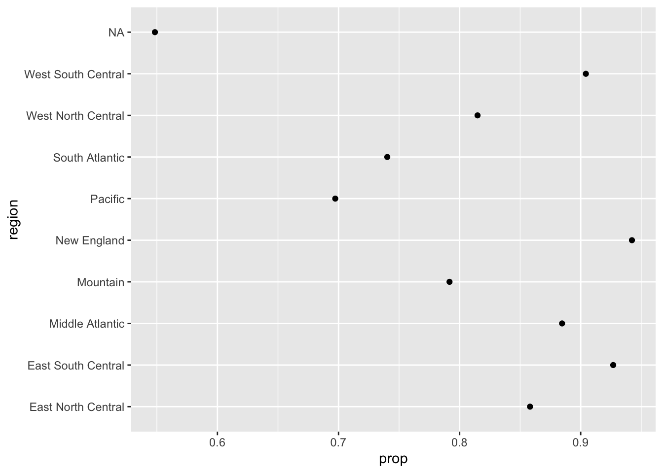
This plot is difficult to read, primarily due to the way the points are ordered. Showing the regions in alphabetical order makes it more difficult to discern the trend. Instead, we would likely wish to reorder this variable by the ascending order of the proportion that check the weather. We will use the fct_reorder function from the forcats package. Note, I also omit the NA category here.
ggplot(na.omit(prop_check_weather),
       aes(prop, fct_reorder(region, prop))) +
  geom_point()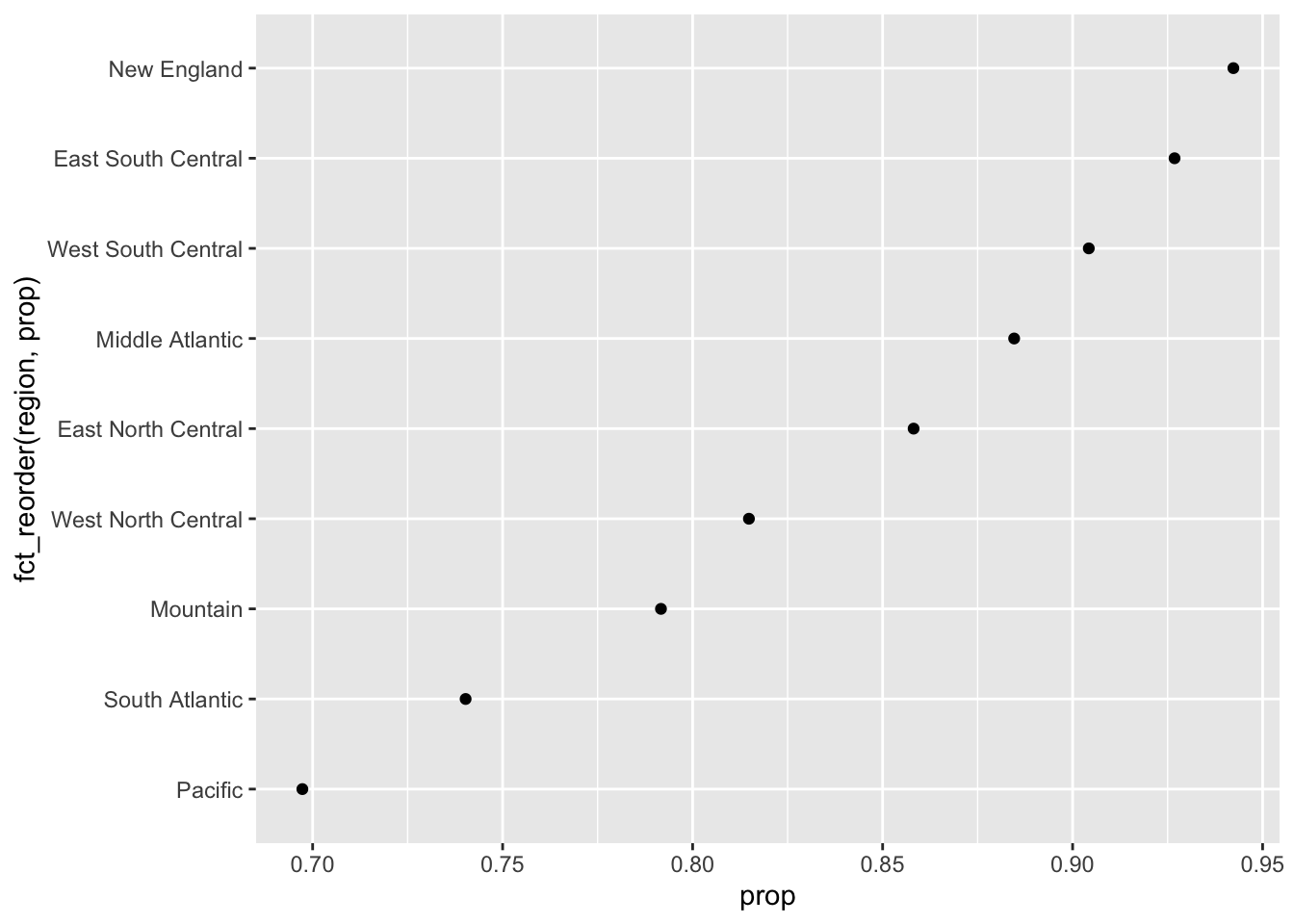
Need to be a bit careful with this operation however. For example:
weather_check %>%
  group_by(hhold_income) %>%
  summarise(prop = mean(ck_weather)) %>%
  na.omit() %>%
  ggplot(aes(prop, fct_reorder(hhold_income, prop))) +
  geom_point()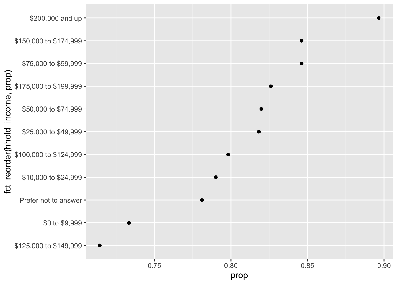
Instead, this is the proper way to show this relationship:
weather_check %>%
  group_by(hhold_income) %>%
  summarise(prop = mean(ck_weather)) %>%
  na.omit() %>%
  ggplot(aes(prop, hhold_income)) +
  geom_point()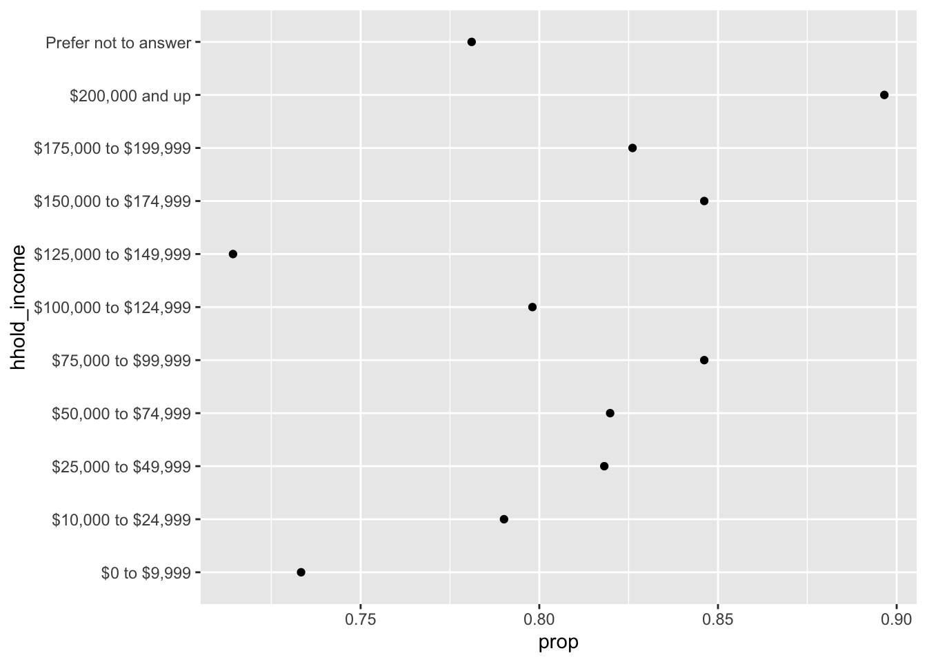
Exercises
- Using data from the
fivethirtyeightpackage calledflying, explore the proportion of respondents that believe the reclining the chair while flying should be eliminated (the variable is recline_eliminate). - Do these proportions differ by the location?
- Create a graphic that captures this relationship, you may wish to reorder the columns to more appropriately represent the relationship.
Rename Factor Levels
These operations are useful to collapse categories or rename levels for publication. The primary function we will use for this operation is fct_recode from the forcats package.
Again, using the weather_check data, suppose we wished to change the levels of the age variable. The levels currently are:
levels(weather_check$age)## [1] "18 - 29" "30 - 44" "45 - 59" "60+"Suppose we wished to better represent these as words. We can use this with mutate from dplyr combined with fct_recode:
weather_check %>%
  mutate(age_recode = fct_recode(age,
      '18 to 29' = '18 - 29',
      '30 to 44' = '30 - 44',
      '45 to 59' = '45 - 59'
  )) %>%
  count(age_recode)
## # A tibble: 5 × 2
## age_recode n
## <fct> <int>
## 1 18 to 29 176
## 2 30 to 44 204
## 3 45 to 59 278
## 4 60+ 258
## 5 <NA> 12We could also collapse categories by assigning many levels to the same new level. For example, suppose we wished to collapse the ck_weather_watch variable to unlikely and likely instead of the very unlikely to very likely.
levels(weather_check$ck_weather_watch)## [1] "Very unlikely" "Somewhat unlikely" "Somewhat likely"
## [4] "Very likely"weather_check %>%
mutate(watch_recode = fct_recode(ck_weather_watch,
'Unlikely' = 'Very unlikely',
'Unlikely' = 'Somewhat unlikely',
'Likely' = 'Somewhat likely',
'Likely' = 'Very likely'
)) %>%
count(watch_recode)## # A tibble: 3 × 2
## watch_recode n
## <ord> <int>
## 1 Unlikely 281
## 2 Likely 636
## 3 <NA> 11Finally, one last option that may be useful is to lump together categories that are too small to report independently. This functionality is implemented with the function fct_lump. For example, suppose we want to lump the region variable together to have only 5 regions.
weather_check %>%
  mutate(region = fct_lump(region, n = 5)) %>%
  count(region, sort = TRUE)
## # A tibble: 7 × 2
## region n
## <fct> <int>
## 1 Other 219
## 2 Pacific 185
## 3 South Atlantic 154
## 4 East North Central 141
## 5 Middle Atlantic 104
## 6 West South Central 94
## 7 <NA> 31Exercises
- Again, using the
flyingdata from thefivethirtyeightpackage, is there a relationship between the proportion of respondents who have a children under 18 years old and if they believe it is rude to bring a baby on a plane? For this question, collapse the baby variable to two levels, no and yes.