ggplot2 extensions
The ggplot2 package has a robust ecosystem of many other packages that extend the functionality of ggplot2. This week, we are going to explore some of these packages in more detail, highlighting a few packages that give you additional ways to create stunning visualizations. You can see all of the extensions packages in the following ggplot2 extension website.
We are going to spend some time with the following packages:
I also plan to discuss, gganimate, but we are going to come back to this later in the course when talking about interactive graphics.
All of these packages are on CRAN and you can install with the following command:
install.packages(c("ggrepel", "ggforce", "patchwork"))ggrepel
Let’s start by exploring the ggrepel package. This package is particularly useful when working with text labels and provides some algorithms to help with text label placement automatically. One challenge when placing text labels in a figure is that they often overlap and they also often are placed on top of the data too. ggrepel helps to solve this problem.
To show a motivating example, we are going to use data in this section based on penguins. To do this, we first need to install this data package.
install.packages("palmerpenguins")The data include three different species of penguins originally collected by Dr. Kristen Gorman at the Palmer Station in Antarctica. There are a total of 344 penguins collected from 3 islands in Antarctica and include information about the species, which island, penguin measurements, and the sex of the penguin. More information about the data including artwork about the species and penguin measurements are on this page.
Here are the penguin species and what the measurements mean, “artwork by @allison_horst”.
library(palmerpenguins)
library(ggplot2)

penguins
## # A tibble: 344 × 8
## species island bill_length_mm bill_depth_mm flipper_length_mm body_mass_g
## <fct> <fct> <dbl> <dbl> <int> <int>
## 1 Adelie Torgersen 39.1 18.7 181 3750
## 2 Adelie Torgersen 39.5 17.4 186 3800
## 3 Adelie Torgersen 40.3 18 195 3250
## 4 Adelie Torgersen NA NA NA NA
## 5 Adelie Torgersen 36.7 19.3 193 3450
## 6 Adelie Torgersen 39.3 20.6 190 3650
## 7 Adelie Torgersen 38.9 17.8 181 3625
## 8 Adelie Torgersen 39.2 19.6 195 4675
## 9 Adelie Torgersen 34.1 18.1 193 3475
## 10 Adelie Torgersen 42 20.2 190 4250
## # … with 334 more rows, and 2 more variables: sex <fct>, year <int>Suppose we wanted to explore the bill length and flipper length with a scatter plot. We can do that with ggplot2 using the geom_point() function. I’m also using the theme_set() function to set the theme to be theme_bw() for the remainder of the notebook. I’ve also altered the theme settings by increasing the base font size from 12 to 16 so hopefully it is a bit easier to read the figure.
theme_set(theme_bw(base_size = 16))

ggplot(penguins, aes(x = flipper_length_mm, y = bill_length_mm)) +
  geom_point(size = 4) +
  xlab("Penguin Flipper Length (in mm)") +
  ylab("Penguin Bill Length (in mm)")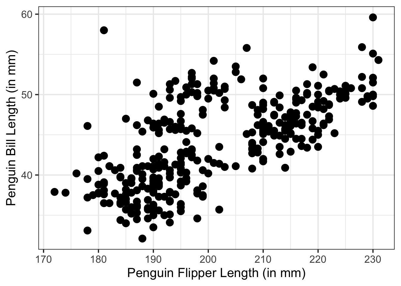
Suppose we wished to add the species to this figure. More specifically, we want to add the species information to the points in the figure to label which points below to each penguin species. There are a few ways we could do this, we could do this by color, shape, or both.
ggplot(penguins, aes(x = flipper_length_mm, y = bill_length_mm)) +
  geom_point(size = 4, aes(color = species, shape = species)) +
  xlab("Penguin Flipper Length (in mm)") +
  ylab("Penguin Bill Length (in mm)")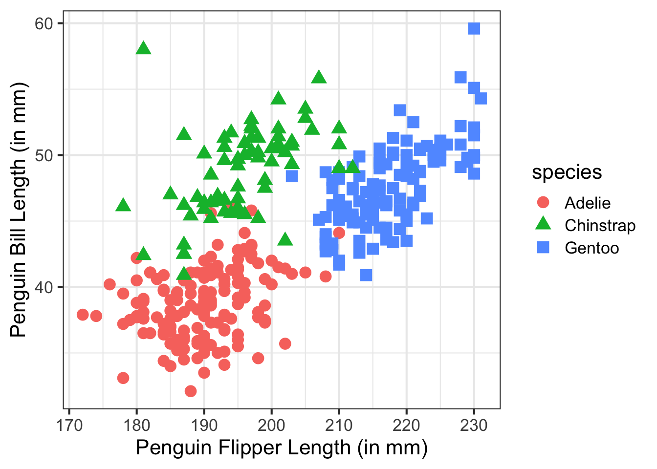
Another potential option would be to add the text labels directly to the figure and not use color. Adding text to a figure is typically done with the geom_text() function.
ggplot(penguins, aes(x = flipper_length_mm, y = bill_length_mm)) +
  geom_point(size = 4, aes(shape = species)) +
  geom_text(aes(label = species)) +
  xlab("Penguin Flipper Length (in mm)") +
  ylab("Penguin Bill Length (in mm)")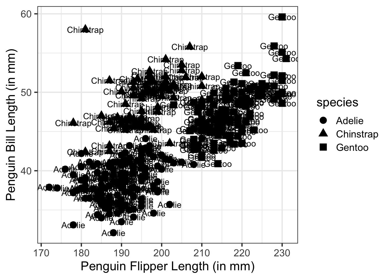
Notice how the text labels overlap and the word is centered with the data point? This makes the plot unusable. We could fiddle with some settings to the geom_text() function, but the ggrepel package helps to fix this issue for us without having to guess and test. The primary difference in the code below is to use geom_text_repel() instead of geom_text(). Note, I shrunk the data point slightly in the following figure.
library(ggrepel)

ggplot(penguins, aes(x = flipper_length_mm, y = bill_length_mm)) +
  geom_point(size = 3, aes(shape = species)) +
  geom_text_repel(aes(label = species)) +
  xlab("Penguin Flipper Length (in mm)") +
  ylab("Penguin Bill Length (in mm)")
This isn’t actually better, but you can see the points were moved away. The issue here is that there are too many text labels to show in a single plot. I’m going to plot only 30 points, 10 from each species.
library(dplyr)
set.seed(100)

penguins %>%
  group_by(species) %>%
  sample_n(10) %>%
  ggplot(., aes(x = flipper_length_mm, y = bill_length_mm)) +
  geom_point(size = 3, aes(shape = species)) +
  geom_text_repel(aes(label = species)) +
  xlab("Penguin Flipper Length (in mm)") +
  ylab("Penguin Bill Length (in mm)")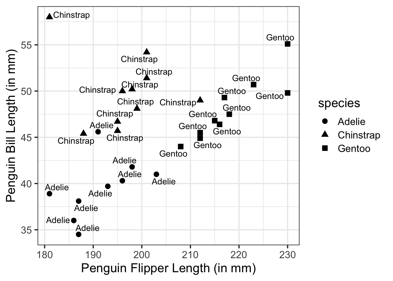
To see exactly what was done, I’m going to generate the same figure using geom_text().
set.seed(100)

penguins %>%
  group_by(species) %>%
  sample_n(10) %>%
  ggplot(., aes(x = flipper_length_mm, y = bill_length_mm)) +
  geom_point(size = 3, aes(shape = species)) +
  geom_text(aes(label = species)) +
  xlab("Penguin Flipper Length (in mm)") +
  ylab("Penguin Bill Length (in mm)")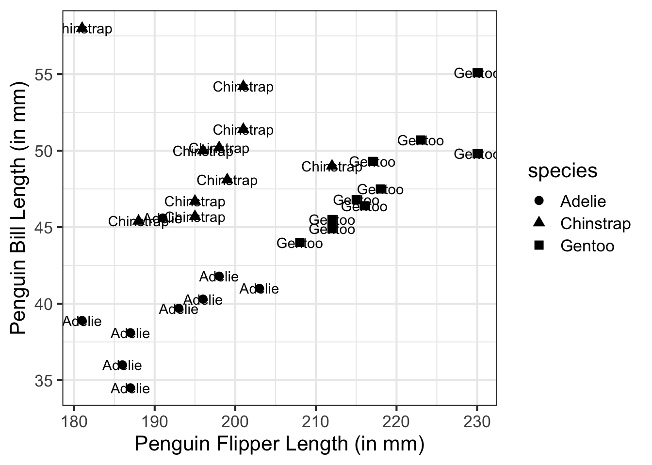
geom_label_repel()
The ggrepel package only has two functions, the first we saw, geom_text_repel(). The second is geom_label_repel(). This works the same as geom_text_repel(), but creates a box around the text attribute.
set.seed(100)

penguins %>%
  group_by(species) %>%
  sample_n(10) %>%
  ggplot(., aes(x = flipper_length_mm, y = bill_length_mm)) +
  geom_point(size = 3, aes(shape = species)) +
  geom_label_repel(aes(label = species)) +
  xlab("Penguin Flipper Length (in mm)") +
  ylab("Penguin Bill Length (in mm)")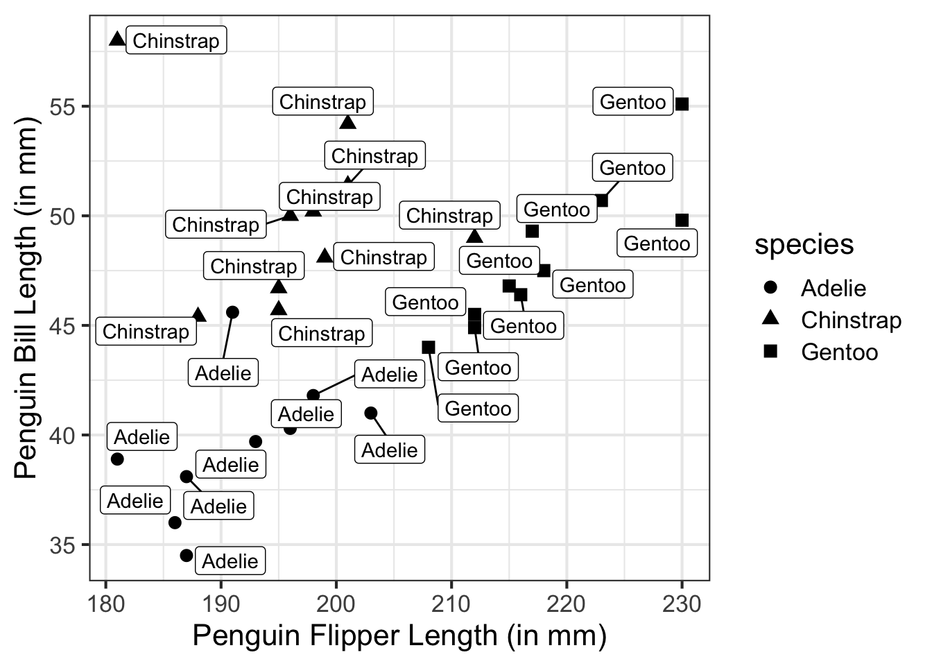
ggforce
The ggforce package has a few powerful additions. One of these helps to solve the problem of too many text labels when using the entire penguin data and is the problem I’d like to start with.
ggplot(penguins, aes(x = flipper_length_mm, y = bill_length_mm)) +
  geom_point(size = 3, aes(shape = species)) +
  geom_text_repel(aes(label = species)) +
  xlab("Penguin Flipper Length (in mm)") +
  ylab("Penguin Bill Length (in mm)")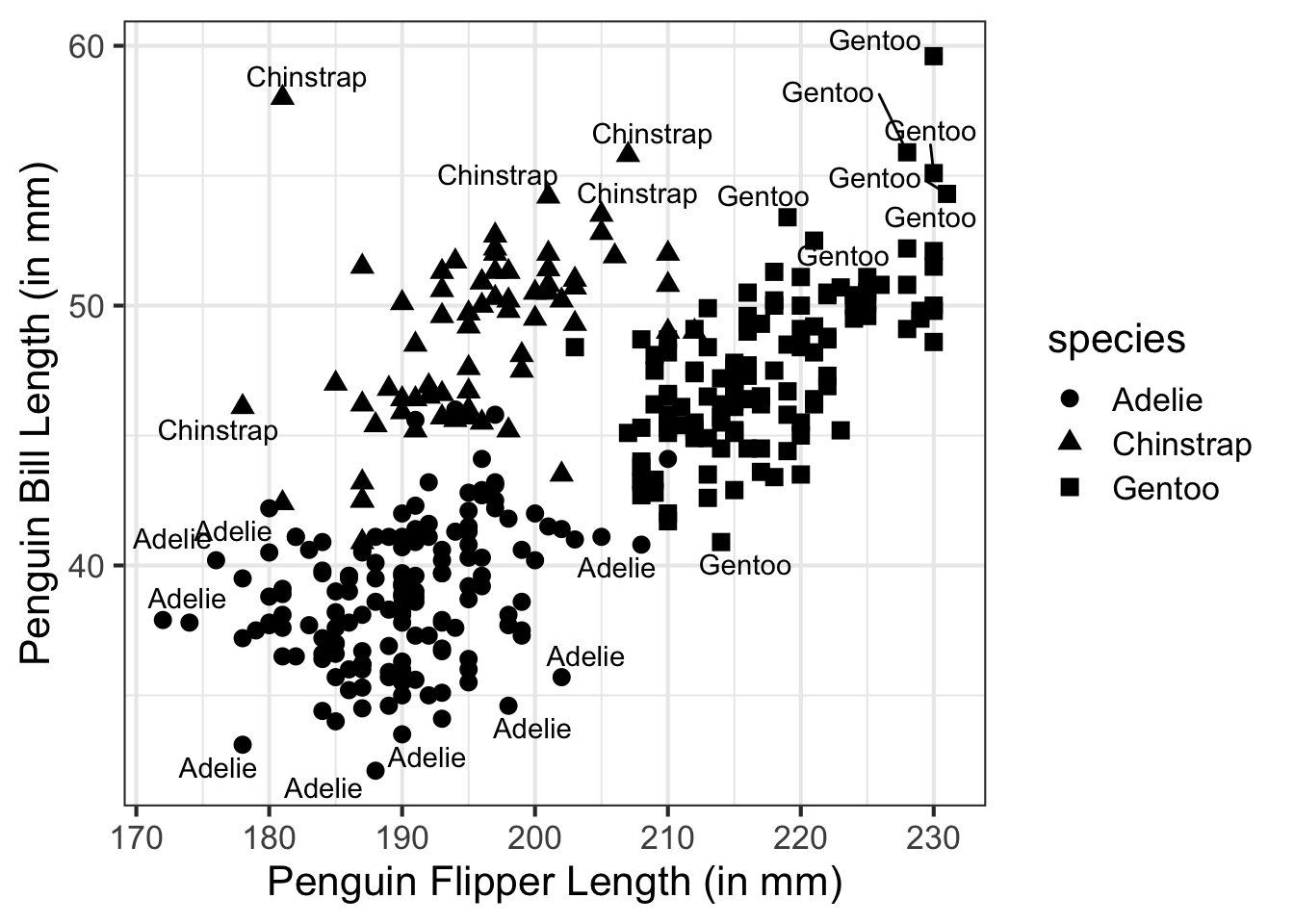
Way too many text labels and for this example, there would be too many duplicate text labels. Since there are only three species, other ways of showing the text and groups would be helpful. ggforce helps with this problem using a series of functions that enclose data within different shapes. These functions are geom_mark_rect(), geom_mark_circle(), geom_mark_ellipse(), and geom_mark_hull() for rectangle, circle, ellipse, and hulls respectively. For an example, let’s try geom_mark_ellipse() instead of the text labels.
library(ggforce)
library(tidyr)

penguins %>%
  drop_na(flipper_length_mm, bill_length_mm) %>%
ggplot(., aes(x = flipper_length_mm, y = bill_length_mm)) +
  geom_mark_ellipse(aes(fill = species)) +
  geom_point(size = 3, aes(shape = species)) +
  xlab("Penguin Flipper Length (in mm)") +
  ylab("Penguin Bill Length (in mm)")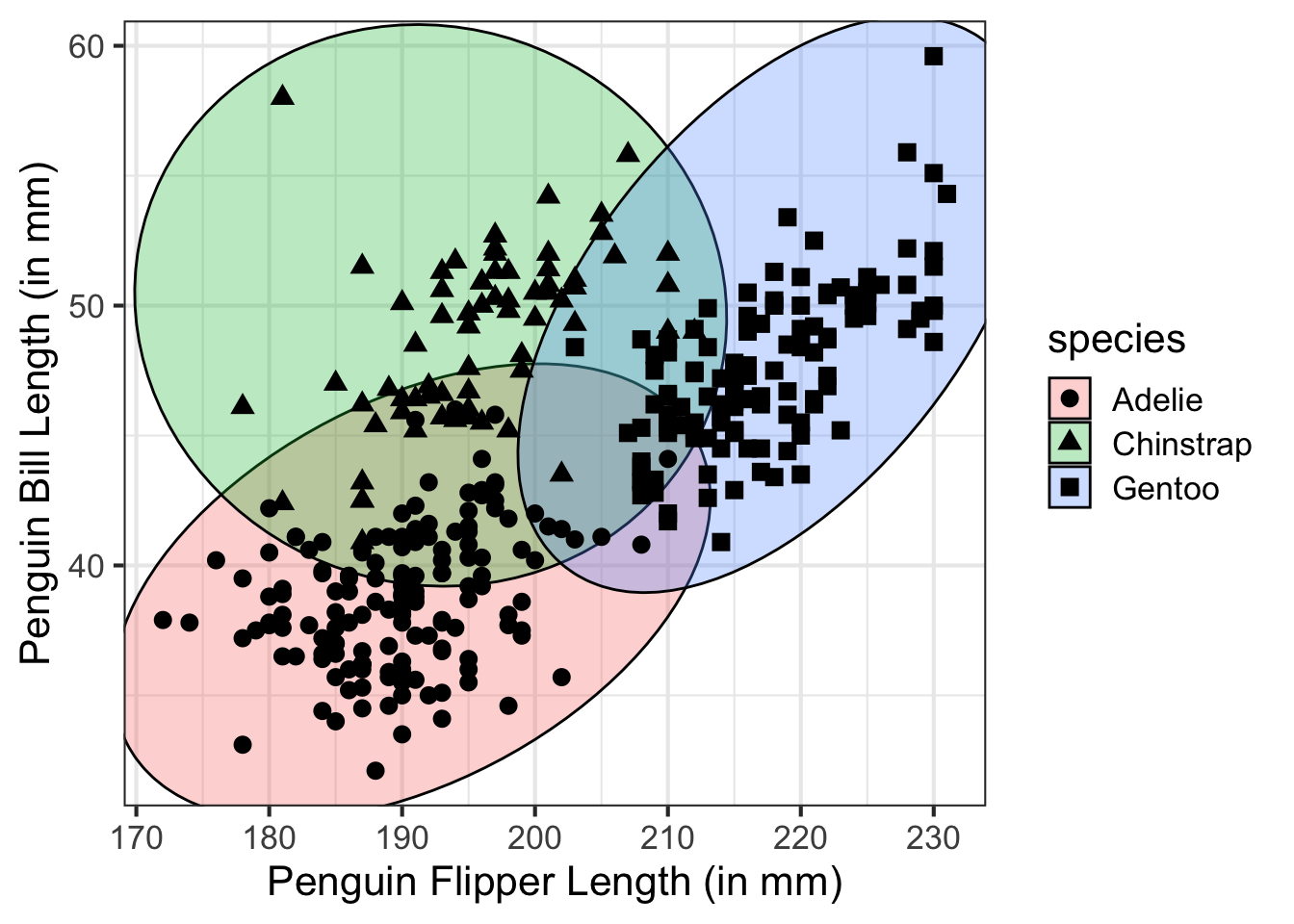
To take this one step further, we can add a text label to this figure by setting a label aesthetic to geom_mark_ellipse().
penguins %>%
  drop_na(flipper_length_mm, bill_length_mm) %>%
  ggplot(., aes(x = flipper_length_mm, y = bill_length_mm)) +
  geom_mark_ellipse(aes(fill = species, label = species)) +
  geom_point(size = 3, aes(shape = species)) +
  scale_x_continuous("Penguin Flipper Length (in mm)") +
  scale_y_continuous("Penguin Bill Length (in mm)",
                     limits = c(25, 70))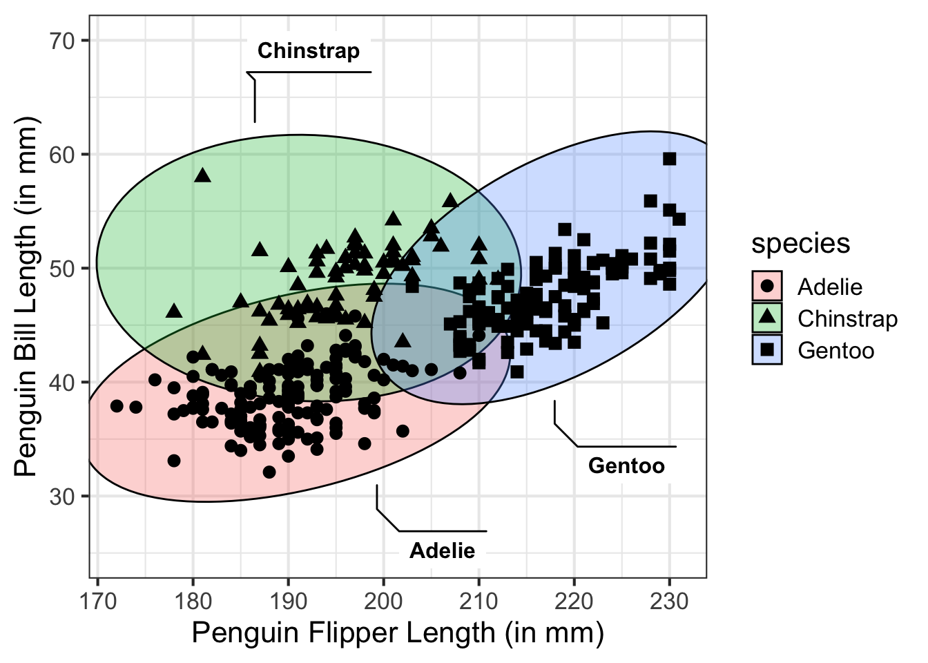
Another cool feature of ggforce is the ability to use something called facet zoom. Essentially, this will create a zoomed in element of a portion of your figure. For example, suppose we wanted to zoom in on the Gentoo penguins to explore their relationship between bill length and flipper length. This creates a picture in picture plotting effect.
ggplot(penguins, aes(x = flipper_length_mm, y = bill_length_mm)) +
  geom_point(size = 3, aes(shape = species, color = species)) +
  xlab("Penguin Flipper Length (in mm)") +
  ylab("Penguin Bill Length (in mm)") +
  facet_zoom(x = species == 'Gentoo')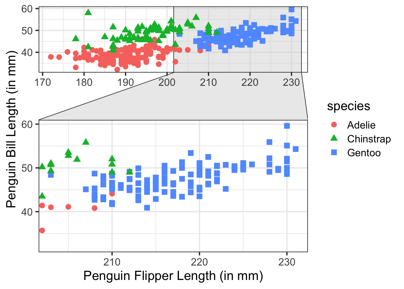
patchwork
The patchwork package is particularly helpful to combine multiple ggplot2 figures into a single figure, but you don’t want to facet. This can be useful to show multiple different relationships of attributes and combine these into a single figure element to include in a document to share.
To combine figure elements, basic math notation is used, including +, /, or |. There are other operators as well, but these are the primary ones we will explore and will also use parentheses to group plots together.
First, let’s create a few plots that we may want to combine.
p1 <- ggplot(penguins, aes(x = flipper_length_mm, y = bill_length_mm)) +
  geom_point(size = 4, aes(color = species, shape = species)) +
  xlab("Penguin Flipper Length (in mm)") +
  ylab("Penguin Bill Length (in mm)")

p1 
p2 <- ggplot(penguins, aes(x = flipper_length_mm, y = bill_depth_mm)) +
  geom_point(size = 4, aes(color = species, shape = species)) +
  xlab("Penguin Flipper Length (in mm)") +
  ylab("Penguin Bill Depth (in mm)")
p2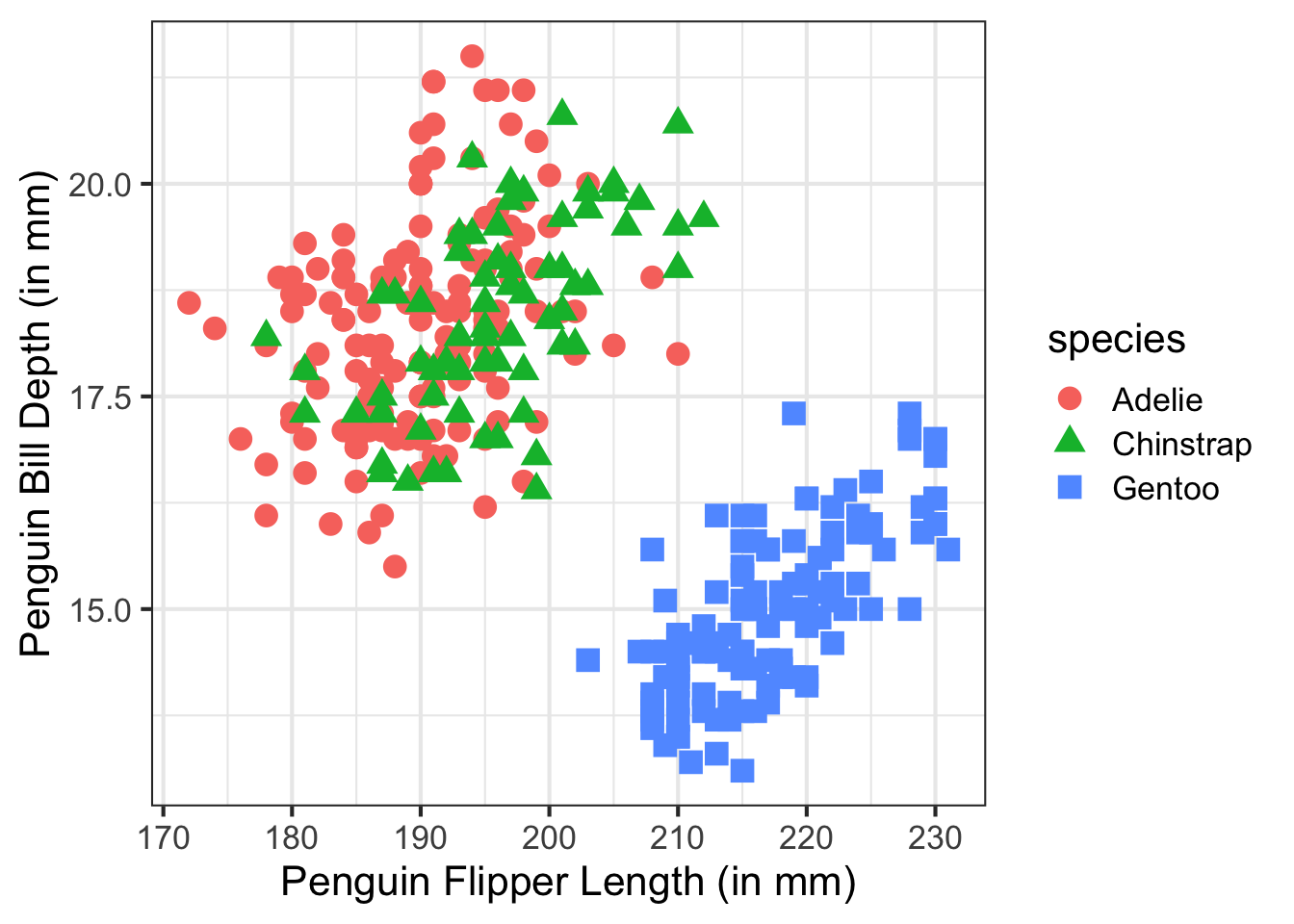
Now, we will start by using the + operator to combine plots.
library(patchwork)

p1 + p2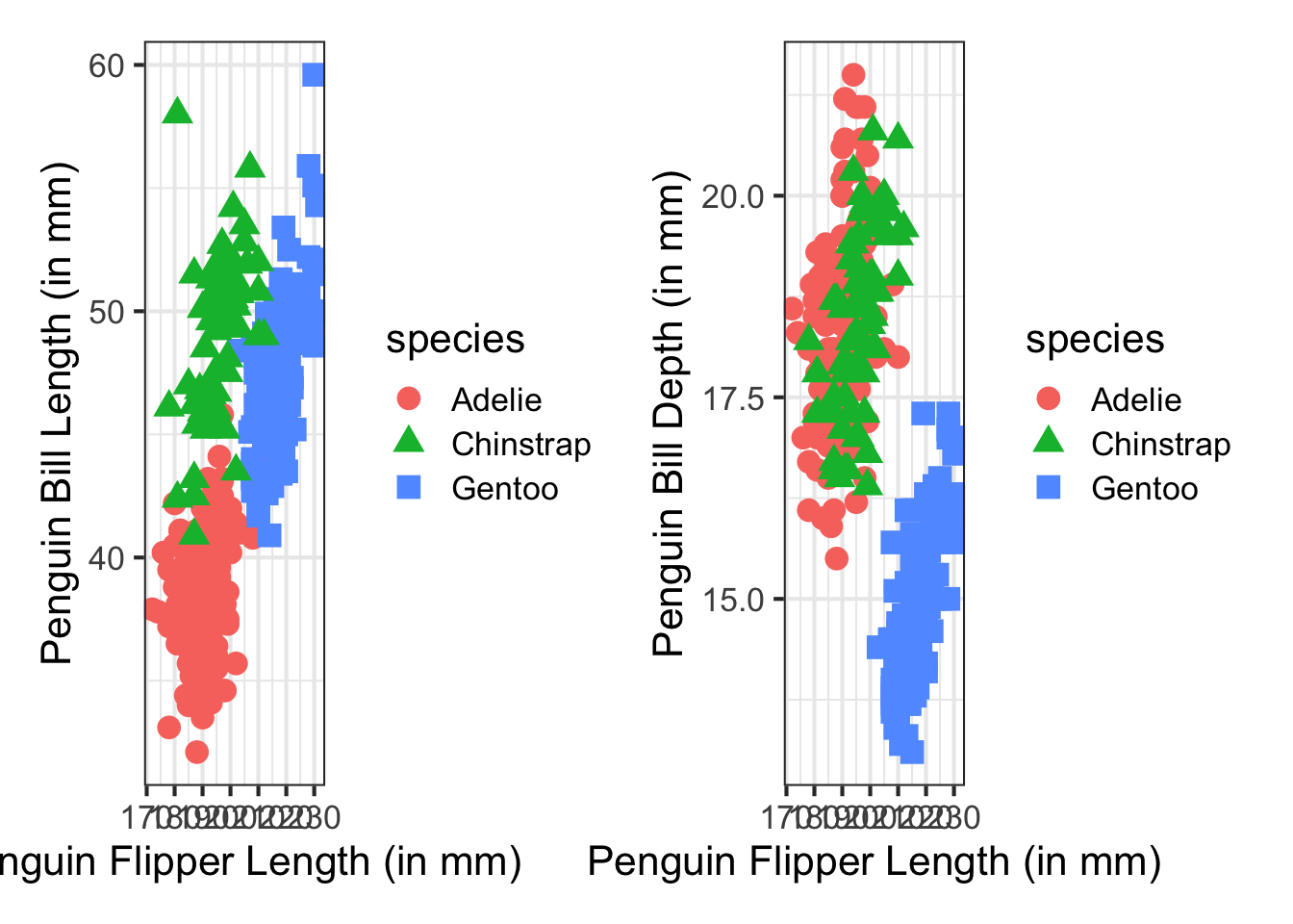
As you can see, the plots are combined directly as generated. In the above example, we’d likely want to only have one legend instead of two. We can do this by modifying the first figure to remove the legend.
p1 <- ggplot(penguins, aes(x = flipper_length_mm, y = bill_length_mm)) +
  geom_point(size = 4, aes(color = species, shape = species)) +
  xlab("Penguin Flipper Length (in mm)") +
  ylab("Penguin Bill Length (in mm)") +
  theme(legend.position = 'none')

p1 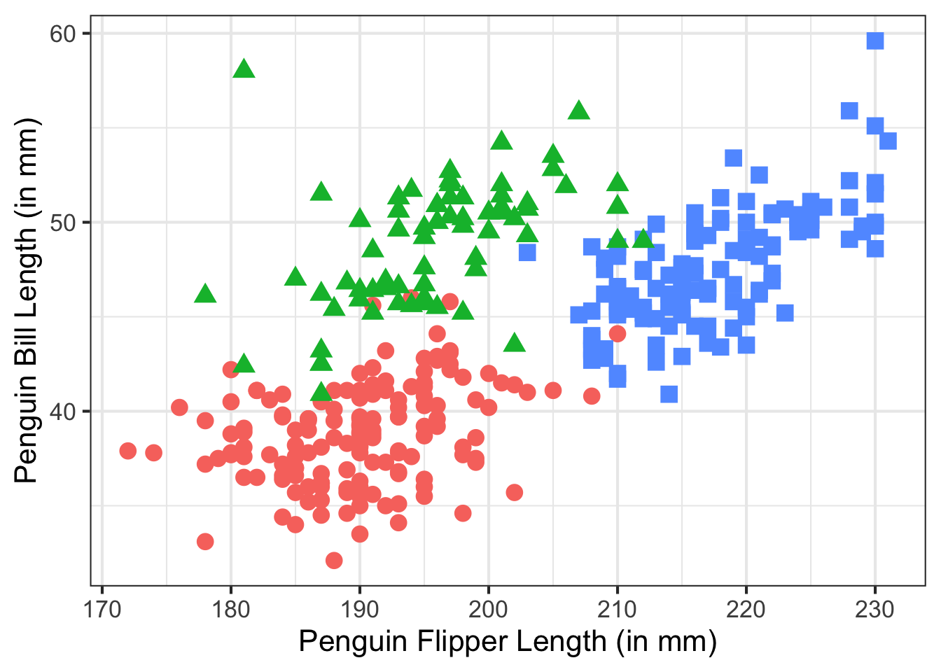
p1 + p2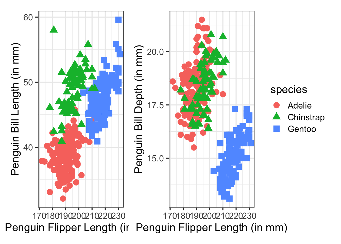
We can use the / operator to stack plots into multiple rows.
p1 / p2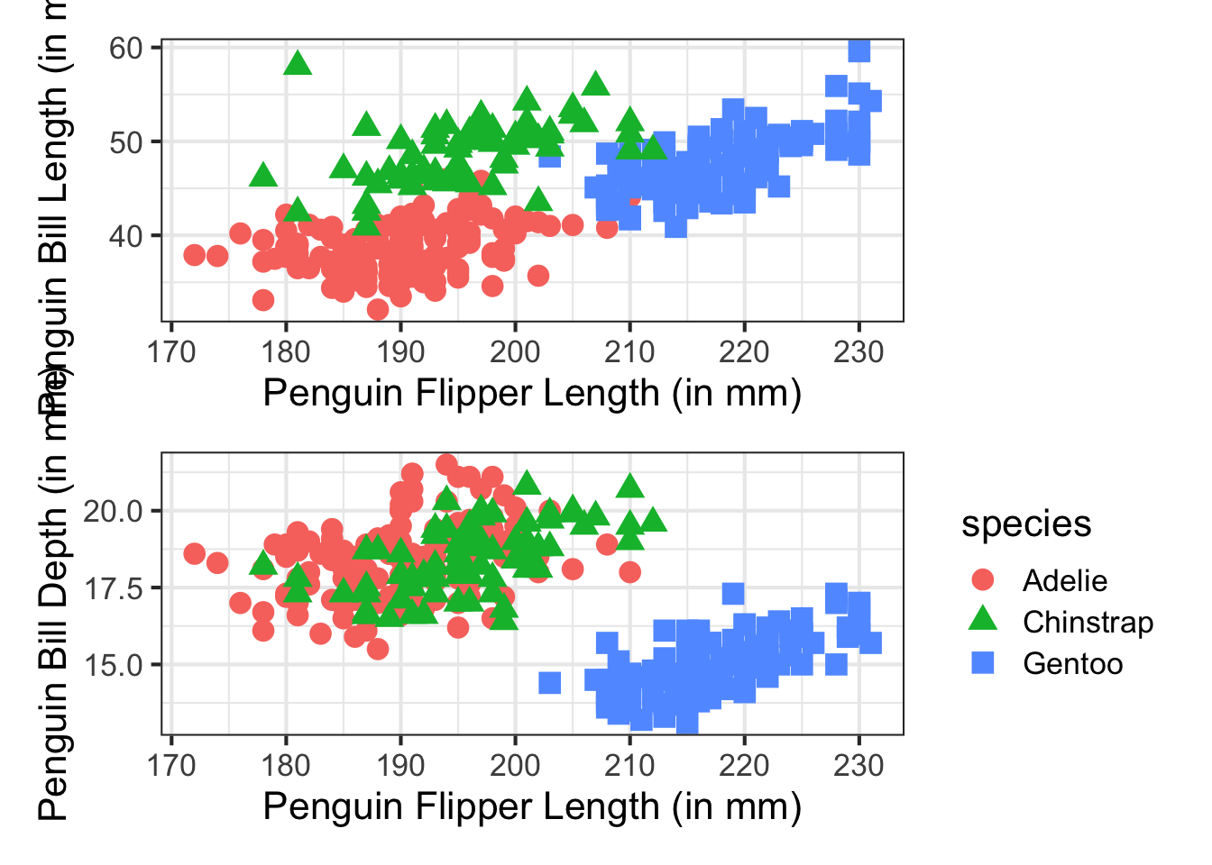
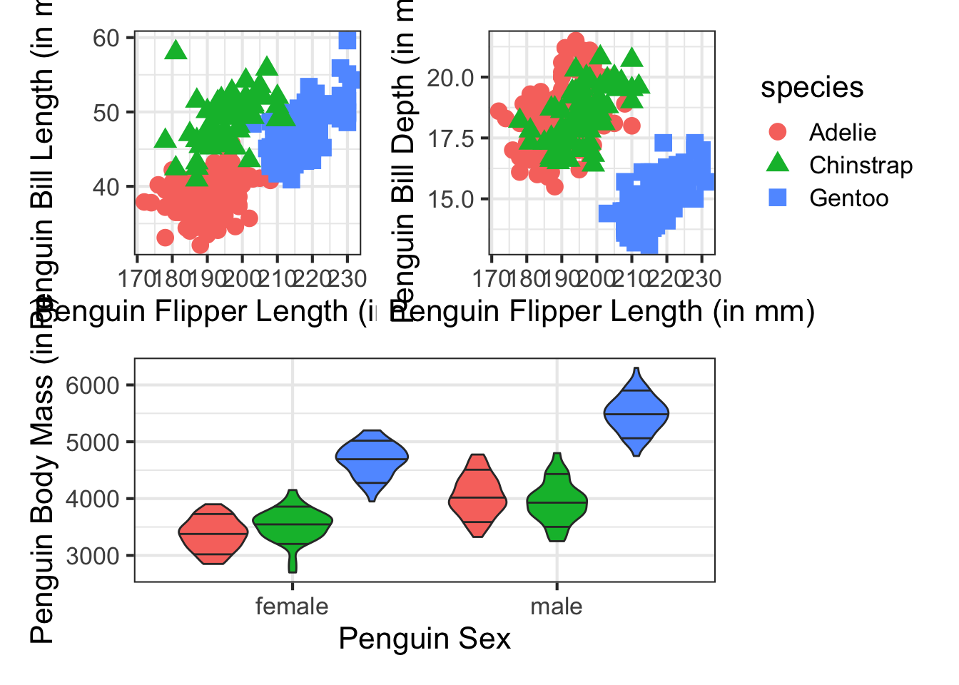
The + operator has one issue with it, it tries to keep things in a square grid, similar to how facet_wrap() works. For more advanced layout, the | operator separates columns whereas we saw above that the / operator will stack plots. Combined with parentheses, you can get more advanced layouts. First, let’s add one more figure.
p3 <- ggplot(drop_na(penguins, sex),
             aes(x = sex, y = body_mass_g)) +
  geom_violin(aes(fill = species), draw_quantiles = c(0.1, .5, 0.9)) +
  xlab("Penguin Sex") +
  ylab("Penguin Body Mass (in g)") +
  theme(legend.position = 'none')

p3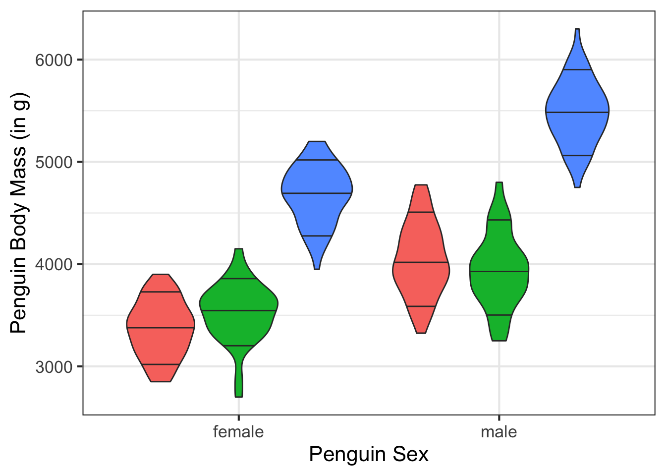
p3 | (p1 / p2)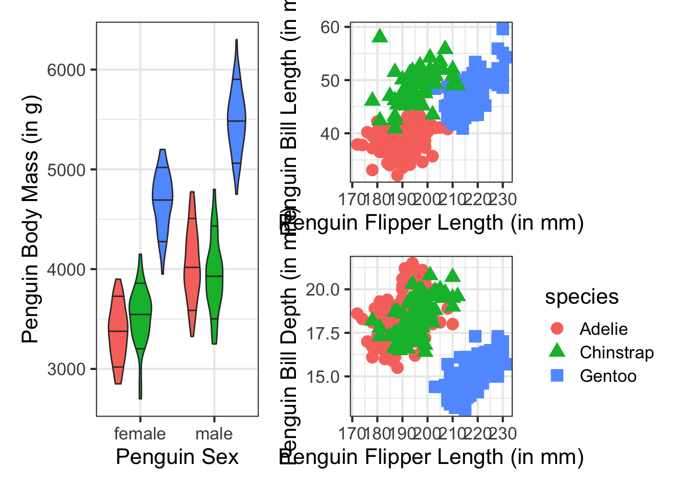
Note, without parentheses, the figures may not turn out as you want.
p1 | p2 / p3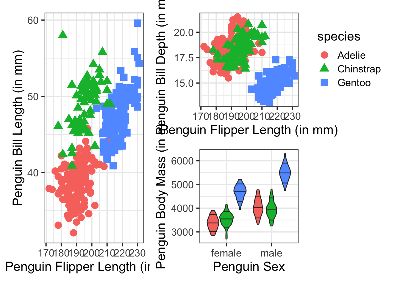
(p1 + p2) / p3