Miscellaneous Modeling Topics
I want to spend a little bit of time talking about ways to model non-linear trends within a linear model as well as show an example of conducting a logistic regression within R using the glm function. This set of notes will use the following packages:
library(modelr)
library(broom)
library(forcats)
library(tidyverse)
Modeling non-linear trends
Modeling non-linear trends can be important and a great way to increase variance explained. There are many ways to model non-linear trends, including non-linear models, but I am going to focus on a linear modeling framework to include non-linear trends by adding quadratic terms.
These types of models are flexible and relatively easy to interpret, however have the drawback that prediction outside of the data at hand (extrapolation) can be problematic. Using the final model from the model assumptions lecture, lets see if we can improve model fit and the trend in the residuals by adding some non-linearity in the form of quadratic terms.
If you recall, here is the model that was used last time.
heights2 <- heights %>%
  mutate(
    marital_comb = fct_recode(marital,
                              'Other' = 'separated',
                              'Other' = 'widowed'
    ),
    income2 = ifelse(income == 0, .001, income),
    height2 = height - mean(height, na.rm = TRUE),
    education2 = education - mean(education, na.rm = TRUE),
    weight2 = weight - mean(weight, na.rm = TRUE),
    log_income = log(income2)
  )
afqt_alt <- lm(afqt ~ marital_comb + height2 + education2 +
                 log_income + weight2, data = heights2)
summary(afqt_alt)
##
## Call:
## lm(formula = afqt ~ marital_comb + height2 + education2 + log_income +
## weight2, data = heights2)
##
## Residuals:
## Min 1Q Median 3Q Max
## -80.466 -16.515 -2.036 16.088 101.730
##
## Coefficients:
## Estimate Std. Error t value Pr(>|t|)
## (Intercept) 32.645765 0.717463 45.502 < 2e-16 ***
## marital_combmarried 9.312248 0.802952 11.598 < 2e-16 ***
## marital_combOther -2.537031 1.231340 -2.060 0.0394 *
## marital_combdivorced 4.790976 0.913836 5.243 1.63e-07 ***
## height2 0.781474 0.077526 10.080 < 2e-16 ***
## education2 5.911616 0.111848 52.854 < 2e-16 ***
## log_income 0.395176 0.038720 10.206 < 2e-16 ***
## weight2 -0.027669 0.007074 -3.911 9.27e-05 ***
## ---
## Signif. codes: 0 '***' 0.001 '**' 0.01 '*' 0.05 '.' 0.1 ' ' 1
##
## Residual standard error: 22.57 on 6637 degrees of freedom
## (361 observations deleted due to missingness)
## Multiple R-squared: 0.3969, Adjusted R-squared: 0.3963
## F-statistic: 624 on 7 and 6637 DF, p-value: < 2.2e-16Let’s see if there are non-linear trends in the height, weight, or income variables. I am going to add these by specifically creating additional variables and using these as new predictors. You could also create these by using the insulate function I() to do the operation within the model syntax.
heights2 <- heights2 %>%
  mutate(
    height2_quad = height2 ^ 2,
    weight2_quad = weight2 ^ 2,
    log_income_quad = log_income ^ 2,
    education2_quad = education2 ^ 2
  )
afqt_alt <- lm(afqt ~ marital_comb + height2 + education2 +
                 log_income + weight2 + education2_quad +
                 height2_quad + weight2_quad + log_income_quad,
               data = heights2)
summary(afqt_alt)
##
## Call:
## lm(formula = afqt ~ marital_comb + height2 + education2 + log_income +
## weight2 + education2_quad + height2_quad + weight2_quad +
## log_income_quad, data = heights2)
##
## Residuals:
## Min 1Q Median 3Q Max
## -77.098 -16.265 -2.331 15.587 91.339
##
## Coefficients:
## Estimate Std. Error t value Pr(>|t|)
## (Intercept) 1.665e+01 1.598e+00 10.419 < 2e-16 ***
## marital_combmarried 8.340e+00 7.993e-01 10.434 < 2e-16 ***
## marital_combOther -2.604e+00 1.218e+00 -2.137 0.0326 *
## marital_combdivorced 4.262e+00 9.061e-01 4.703 2.61e-06 ***
## height2 7.488e-01 7.967e-02 9.399 < 2e-16 ***
## education2 5.467e+00 1.173e-01 46.609 < 2e-16 ***
## log_income -3.828e-01 8.307e-02 -4.609 4.12e-06 ***
## weight2 -4.652e-02 8.046e-03 -5.782 7.72e-09 ***
## education2_quad 5.535e-02 2.488e-02 2.224 0.0262 *
## height2_quad -3.018e-02 1.392e-02 -2.169 0.0302 *
## weight2_quad 4.135e-04 8.359e-05 4.947 7.73e-07 ***
## log_income_quad 2.177e-01 2.018e-02 10.791 < 2e-16 ***
## ---
## Signif. codes: 0 '***' 0.001 '**' 0.01 '*' 0.05 '.' 0.1 ' ' 1
##
## Residual standard error: 22.33 on 6633 degrees of freedom
## (361 observations deleted due to missingness)
## Multiple R-squared: 0.4102, Adjusted R-squared: 0.4092
## F-statistic: 419.3 on 11 and 6633 DF, p-value: < 2.2e-16Alternatively, this model could look like:
afqt_alt <- lm(afqt ~ marital_comb + height2 + education2 +
                 log_income + weight2 + I(education2^2) +
                 I(height2^2) + I(weight2^2) + I(log_income^2),
               data = heights2)
summary(afqt_alt)
##
## Call:
## lm(formula = afqt ~ marital_comb + height2 + education2 + log_income +
## weight2 + I(education2^2) + I(height2^2) + I(weight2^2) +
## I(log_income^2), data = heights2)
##
## Residuals:
## Min 1Q Median 3Q Max
## -77.098 -16.265 -2.331 15.587 91.339
##
## Coefficients:
## Estimate Std. Error t value Pr(>|t|)
## (Intercept) 1.665e+01 1.598e+00 10.419 < 2e-16 ***
## marital_combmarried 8.340e+00 7.993e-01 10.434 < 2e-16 ***
## marital_combOther -2.604e+00 1.218e+00 -2.137 0.0326 *
## marital_combdivorced 4.262e+00 9.061e-01 4.703 2.61e-06 ***
## height2 7.488e-01 7.967e-02 9.399 < 2e-16 ***
## education2 5.467e+00 1.173e-01 46.609 < 2e-16 ***
## log_income -3.828e-01 8.307e-02 -4.609 4.12e-06 ***
## weight2 -4.652e-02 8.046e-03 -5.782 7.72e-09 ***
## I(education2^2) 5.535e-02 2.488e-02 2.224 0.0262 *
## I(height2^2) -3.018e-02 1.392e-02 -2.169 0.0302 *
## I(weight2^2) 4.135e-04 8.359e-05 4.947 7.73e-07 ***
## I(log_income^2) 2.177e-01 2.018e-02 10.791 < 2e-16 ***
## ---
## Signif. codes: 0 '***' 0.001 '**' 0.01 '*' 0.05 '.' 0.1 ' ' 1
##
## Residual standard error: 22.33 on 6633 degrees of freedom
## (361 observations deleted due to missingness)
## Multiple R-squared: 0.4102, Adjusted R-squared: 0.4092
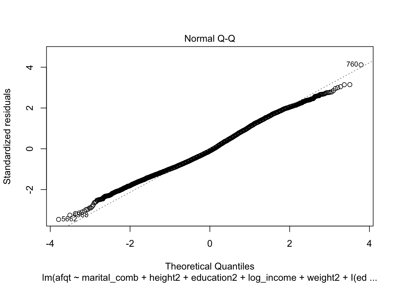
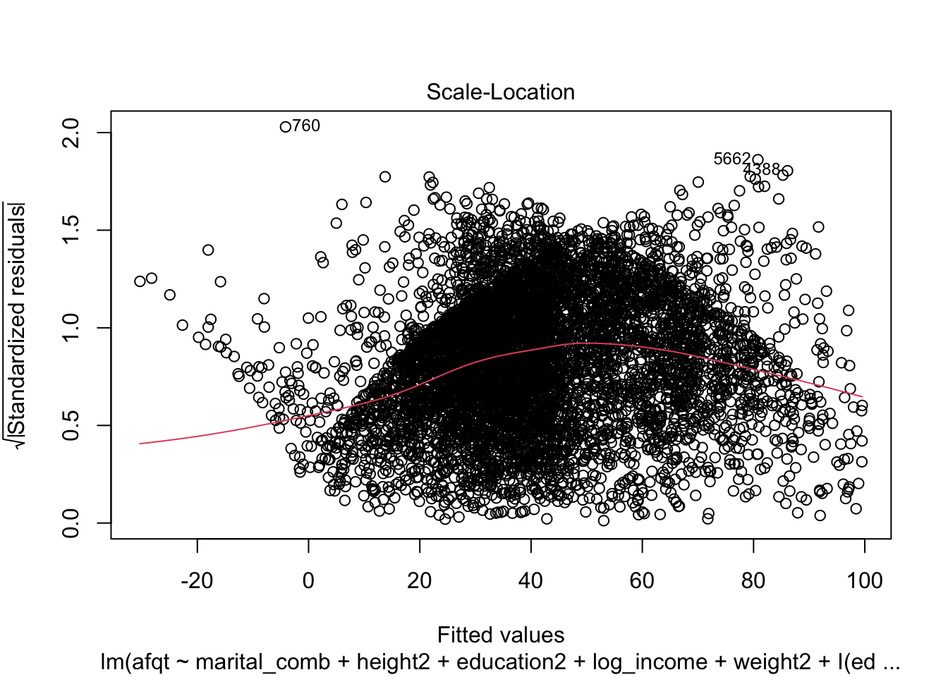
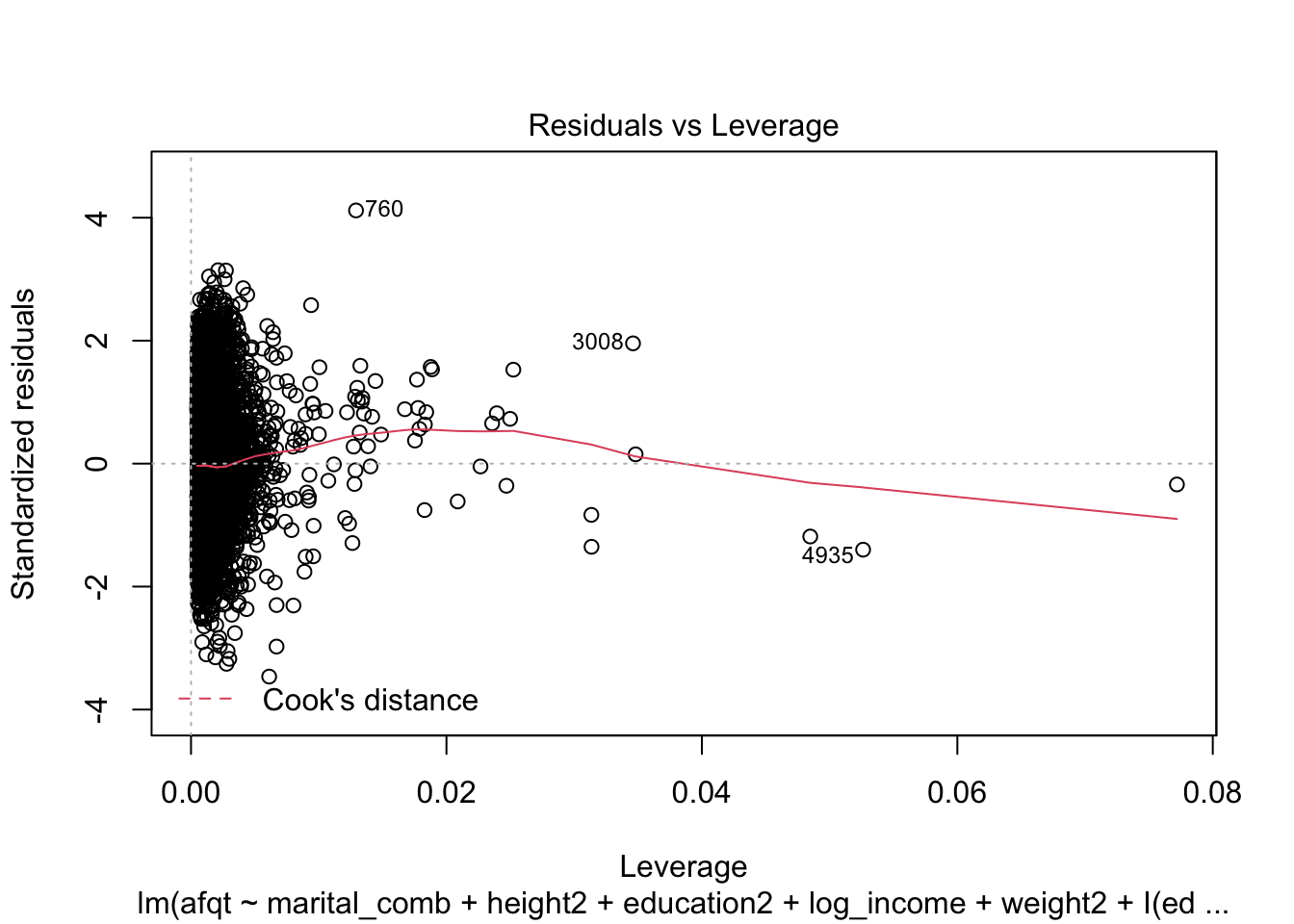
## F-statistic: 419.3 on 11 and 6633 DF, p-value: < 2.2e-16Let’s see if this improved our model fit.
plot(afqt_alt)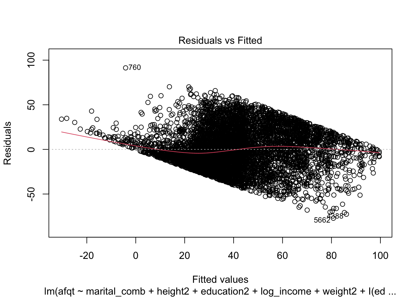
We could also attempt to convert the dependent variable (in a percentile metric) to a z-score.
heights2 <- heights2 %>%
  mutate(
    afqt2 = ifelse(afqt == 0, .00001, ifelse(afqt == 100, 99.9999999, afqt)),
    afqt3 = ifelse(afqt %in% c(0, 100), NA, afqt),
    afqt_z = qnorm(afqt2/100),
    afqt_z3 = qnorm(afqt3/100)
  )
afqt_alt2 <- lm(afqt_z3 ~ marital_comb + height2 + education2 +
                 log_income + weight2 + education2_quad +
                 height2_quad + weight2_quad + log_income_quad,
               data = heights2)
summary(afqt_alt2)
##
## Call:
## lm(formula = afqt_z3 ~ marital_comb + height2 + education2 +
## log_income + weight2 + education2_quad + height2_quad + weight2_quad +
## log_income_quad, data = heights2)
##
## Residuals:
## Min 1Q Median 3Q Max
## -2.8910 -0.5105 -0.0064 0.4966 3.2479
##
## Coefficients:
## Estimate Std. Error t value Pr(>|t|)
## (Intercept) -1.119e+00 5.576e-02 -20.069 < 2e-16 ***
## marital_combmarried 2.942e-01 2.782e-02 10.576 < 2e-16 ***
## marital_combOther -9.070e-02 4.242e-02 -2.138 0.032536 *
## marital_combdivorced 1.701e-01 3.152e-02 5.395 7.09e-08 ***
## height2 2.506e-02 2.769e-03 9.051 < 2e-16 ***
## education2 1.933e-01 4.133e-03 46.769 < 2e-16 ***
## log_income -1.075e-02 2.897e-03 -3.710 0.000209 ***
## weight2 -1.640e-03 2.800e-04 -5.859 4.88e-09 ***
## education2_quad -5.433e-04 8.880e-04 -0.612 0.540682
## height2_quad -1.316e-03 4.838e-04 -2.720 0.006545 **
## weight2_quad 1.508e-05 2.906e-06 5.192 2.15e-07 ***
## log_income_quad 7.100e-03 7.042e-04 10.083 < 2e-16 ***
## ---
## Signif. codes: 0 '***' 0.001 '**' 0.01 '*' 0.05 '.' 0.1 ' ' 1
##
## Residual standard error: 0.7745 on 6588 degrees of freedom
## (406 observations deleted due to missingness)
## Multiple R-squared: 0.4088, Adjusted R-squared: 0.4078
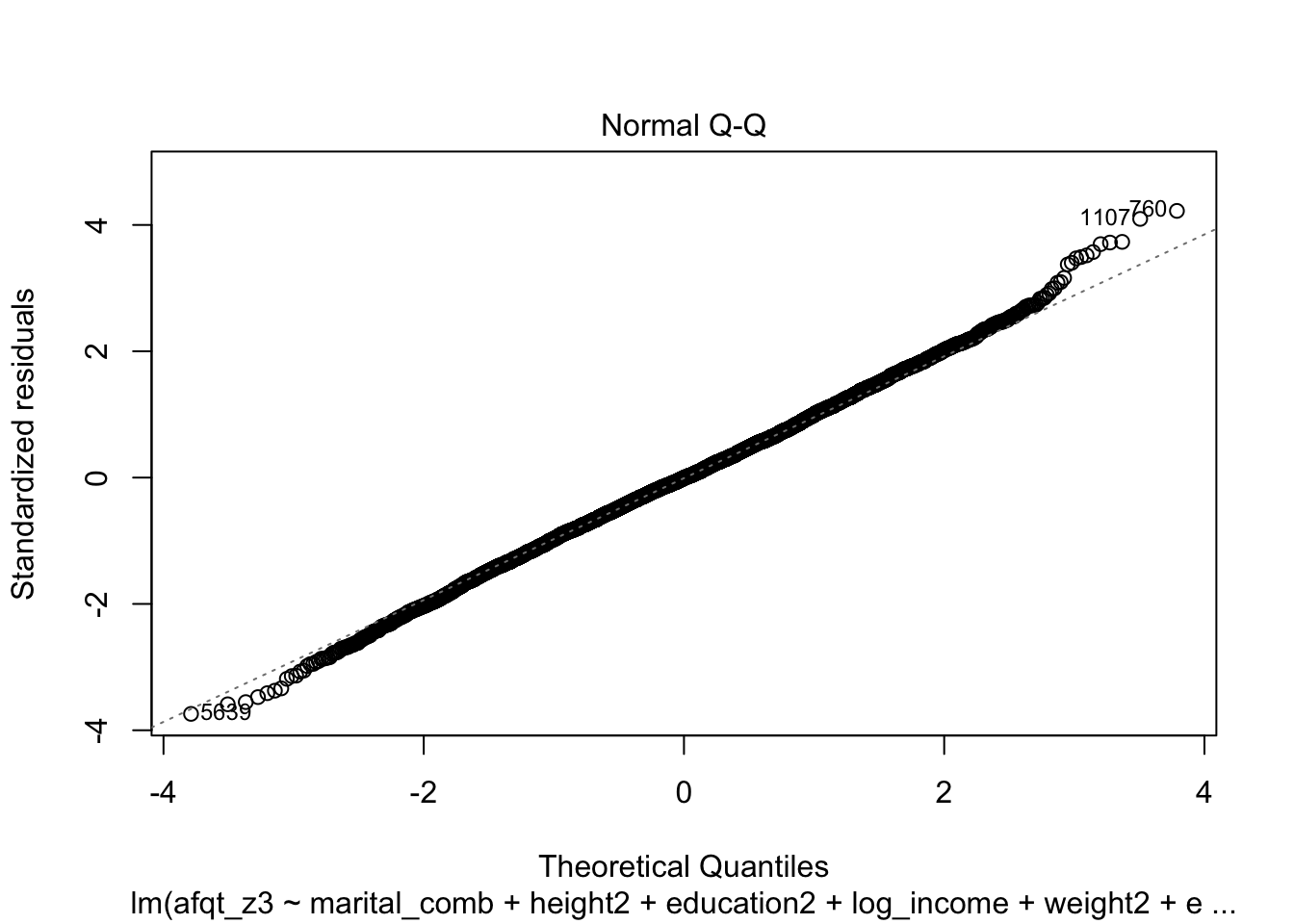
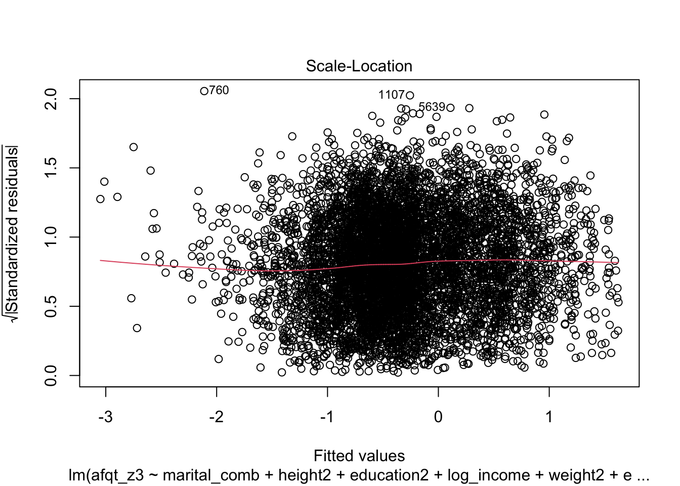
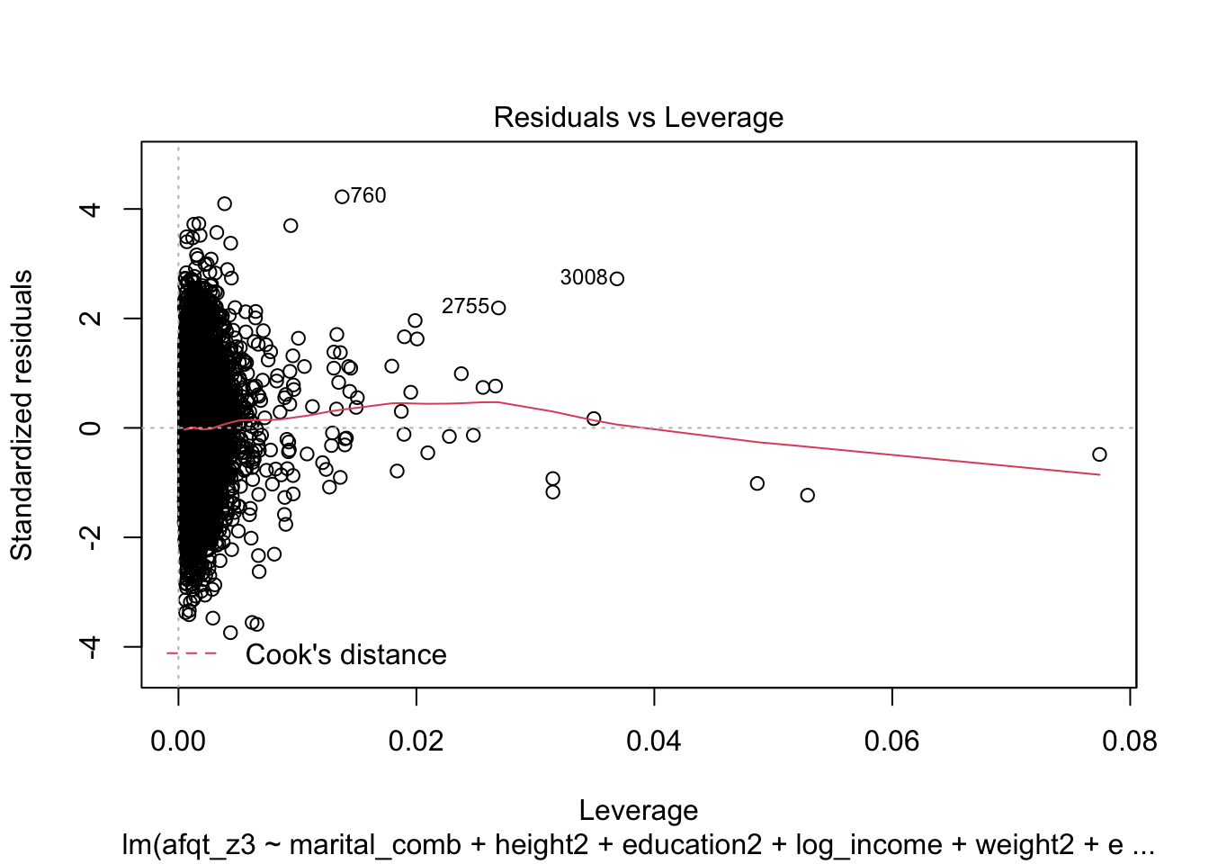
## F-statistic: 414.1 on 11 and 6588 DF, p-value: < 2.2e-16plot(afqt_alt2)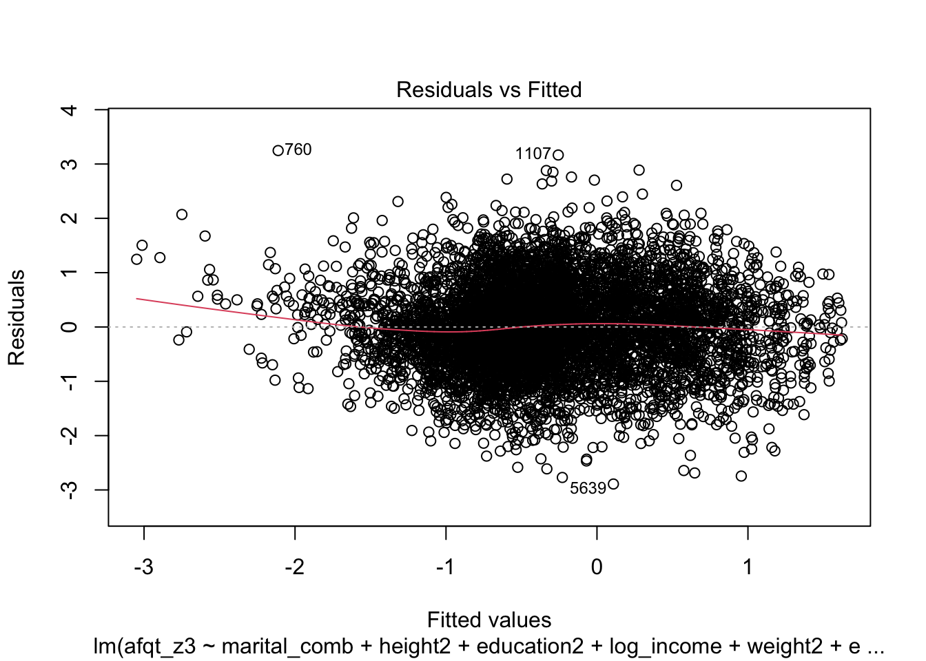
glm function
The glm function behaves much like the lm function. The only major difference in model logistics is that we will now need to specify a family argument. This family argument will depend on the type of model being fitted. We are going to perform a logistic regression, therefore this family will be binomial.
The data we will use is from Kaggle and is data from Titanic, more specifically the data has characteristics on the passengers and whether they survived the shipwreck or not. You can get a sense of the variables from this website: https://www.kaggle.com/c/titanic/data.
library(titanic)

titanic <- bind_rows(titanic_test,
                     titanic_train)
head(titanic)
## PassengerId Pclass Name Sex Age
## 1 892 3 Kelly, Mr. James male 34.5
## 2 893 3 Wilkes, Mrs. James (Ellen Needs) female 47.0
## 3 894 2 Myles, Mr. Thomas Francis male 62.0
## 4 895 3 Wirz, Mr. Albert male 27.0
## 5 896 3 Hirvonen, Mrs. Alexander (Helga E Lindqvist) female 22.0
## 6 897 3 Svensson, Mr. Johan Cervin male 14.0
## SibSp Parch Ticket Fare Cabin Embarked Survived
## 1 0 0 330911 7.8292 Q NA
## 2 1 0 363272 7.0000 S NA
## 3 0 0 240276 9.6875 Q NA
## 4 0 0 315154 8.6625 S NA
## 5 1 1 3101298 12.2875 S NA
## 6 0 0 7538 9.2250 S NASuppose we were interested in fitting a model that predicted whether a passenger survived or not. Using lm is not appropriate as the dependent variable is not continuous, rather it is dichotomous. Using logistic regression is more appropriate here.
surv_mod <- glm(Survived ~ factor(Pclass) + Fare + Sex + Age,
                data = titanic,
                family = binomial)
summary(surv_mod)
##
## Call:
## glm(formula = Survived ~ factor(Pclass) + Fare + Sex + Age, family = binomial,
## data = titanic)
##
## Deviance Residuals:
## Min 1Q Median 3Q Max
## -2.7393 -0.6788 -0.3956 0.6486 2.4639
##
## Coefficients:
## Estimate Std. Error z value Pr(>|z|)
## (Intercept) 3.7225052 0.4645113 8.014 1.11e-15 ***
## factor(Pclass)2 -1.2765903 0.3126370 -4.083 4.44e-05 ***
## factor(Pclass)3 -2.5415762 0.3277677 -7.754 8.89e-15 ***
## Fare 0.0005226 0.0022579 0.231 0.817
## Sexmale -2.5185052 0.2082017 -12.096 < 2e-16 ***
## Age -0.0367302 0.0077325 -4.750 2.03e-06 ***
## ---
## Signif. codes: 0 '***' 0.001 '**' 0.01 '*' 0.05 '.' 0.1 ' ' 1
##
## (Dispersion parameter for binomial family taken to be 1)
##
## Null deviance: 964.52 on 713 degrees of freedom
## Residual deviance: 647.23 on 708 degrees of freedom
## (595 observations deleted due to missingness)
## AIC: 659.23
##
## Number of Fisher Scoring iterations: 5It is common to interpret these in terms of probability, we can do this with the following bit of code:
prob_mod <- titanic %>%
  select(Survived, Pclass, Fare, Sex, Age) %>%
  na.omit() %>%
  mutate(
    probability = predict(surv_mod, type = 'response')
  )

head(prob_mod, n = 15)
## Survived Pclass Fare Sex Age probability
## 419 0 3 7.2500 male 22 0.10509514
## 420 1 1 71.2833 female 38 0.91404126
## 421 1 3 7.9250 female 26 0.55726903
## 422 1 1 53.1000 female 35 0.92162960
## 423 0 3 8.0500 male 35 0.06793029
## 425 0 1 51.8625 male 54 0.32031425
## 426 0 3 21.0750 male 2 0.19781236
## 427 1 3 11.1333 female 27 0.54860408
## 428 1 2 30.0708 female 14 0.87516354
## 429 1 3 16.7000 female 4 0.73937738
## 430 1 1 26.5500 female 58 0.83285937
## 431 0 3 8.0500 male 20 0.11224887
## 432 0 3 31.2750 male 39 0.05987747
## 433 0 3 7.8542 female 14 0.66168470
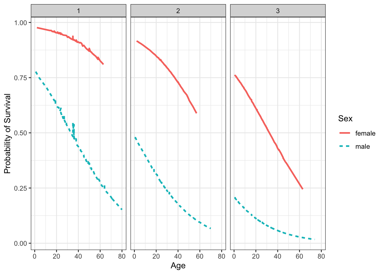
## 434 1 2 16.0000 female 55 0.60685621We could now plot these probabilities to explore the effects.
ggplot(prob_mod, aes(Age, probability, color = Sex, linetype = Sex)) +
  geom_line(size = 1) +
  facet_grid(. ~ Pclass) +
  theme_bw() +
  xlab("Age") +
  ylab("Probability of Survival")