Model Assumptions
I want to spend a little bit of time talking about model assumptions. These are important and should be checked for any analysis. The following packages will be used for this set of notes.
library(modelr)
library(broom)
library(forcats)
library(tidyverse)
We are also going to use this model from the advanced model section to explore model assumptions.
heights2 <- heights %>%
  mutate(
    marital_comb = fct_recode(marital,
          'Other' = 'separated',
          'Other' = 'widowed'
    )
  )

afqt_mod <- lm(afqt ~ marital_comb + height, data = heights2)
summary(afqt_mod)
##
## Call:
## lm(formula = afqt ~ marital_comb + height, data = heights2)
##
## Residuals:
## Min 1Q Median 3Q Max
## -53.150 -22.517 -4.248 22.097 78.355
##
## Coefficients:
## Estimate Std. Error t value Pr(>|t|)
## (Intercept) -28.99932 5.67144 -5.113 3.25e-07 ***
## marital_combmarried 16.13531 0.96385 16.741 < 2e-16 ***
## marital_combOther -4.63978 1.50160 -3.090 0.00201 **
## marital_combdivorced 6.75490 1.11278 6.070 1.35e-09 ***
## height 0.89847 0.08329 10.787 < 2e-16 ***
## ---
## Signif. codes: 0 '***' 0.001 '**' 0.01 '*' 0.05 '.' 0.1 ' ' 1
##
## Residual standard error: 27.78 on 6739 degrees of freedom
## (262 observations deleted due to missingness)
## Multiple R-squared: 0.08467, Adjusted R-squared: 0.08413
## F-statistic: 155.8 on 4 and 6739 DF, p-value: < 2.2e-16plot function with model object
One of the nicest features when model building within R, is that many diagnostic plots are very accessible using the plot function. For example:
plot(afqt_mod)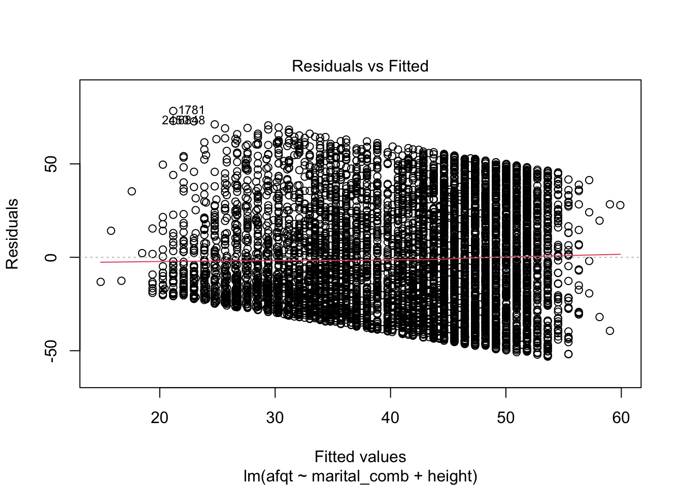
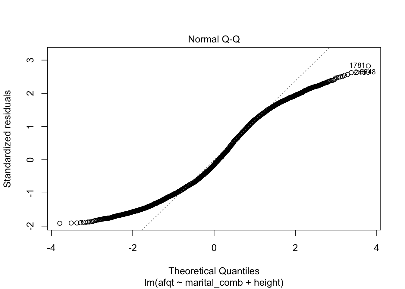
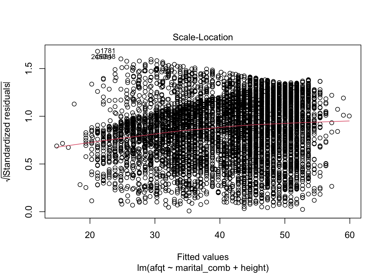
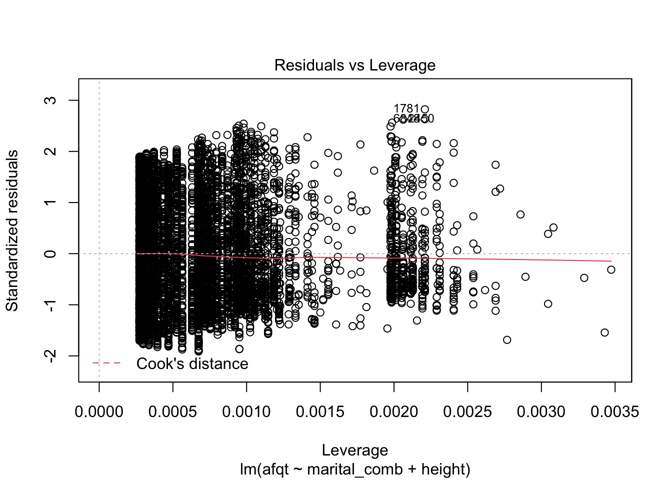
These plots are shown one at a time in an interactive R session, but allow you to check many common assumptions such as normal residuals, linearity, homogeneity of variance, and even leverage.
You can see from these figures that there is quite a bit to be desired from our model. First, the residuals are not normally distributed (very heavy tails) and more problematic is that the residuals have a trend to them. This suggests that we are missing an important variable in the model.
Suppose we add some additional variables to the model keeping the model additive. Note, I am also mean centering many of the continuous variables to ease interpretation slightly.
heights2 <- heights2 %>%
  mutate(income2 = ifelse(income == 0, .001, income),
         height2 = height - mean(height, na.rm = TRUE),
         education2 = education - mean(education, na.rm = TRUE),
         weight2 = weight - mean(weight, na.rm = TRUE),
         log_income = log(income2))
afqt_alt <- lm(afqt ~ marital_comb + height2 + education2 +
                 log_income + weight2, data = heights2)
summary(afqt_alt)
##
## Call:
## lm(formula = afqt ~ marital_comb + height2 + education2 + log_income +
## weight2, data = heights2)
##
## Residuals:
## Min 1Q Median 3Q Max
## -80.466 -16.515 -2.036 16.088 101.730
##
## Coefficients:
## Estimate Std. Error t value Pr(>|t|)
## (Intercept) 32.645765 0.717463 45.502 < 2e-16 ***
## marital_combmarried 9.312248 0.802952 11.598 < 2e-16 ***
## marital_combOther -2.537031 1.231340 -2.060 0.0394 *
## marital_combdivorced 4.790976 0.913836 5.243 1.63e-07 ***
## height2 0.781474 0.077526 10.080 < 2e-16 ***
## education2 5.911616 0.111848 52.854 < 2e-16 ***
## log_income 0.395176 0.038720 10.206 < 2e-16 ***
## weight2 -0.027669 0.007074 -3.911 9.27e-05 ***
## ---
## Signif. codes: 0 '***' 0.001 '**' 0.01 '*' 0.05 '.' 0.1 ' ' 1
##
## Residual standard error: 22.57 on 6637 degrees of freedom
## (361 observations deleted due to missingness)
## Multiple R-squared: 0.3969, Adjusted R-squared: 0.3963
## F-statistic: 624 on 7 and 6637 DF, p-value: < 2.2e-16plot(afqt_alt)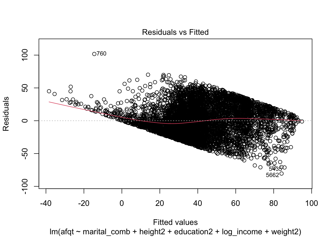
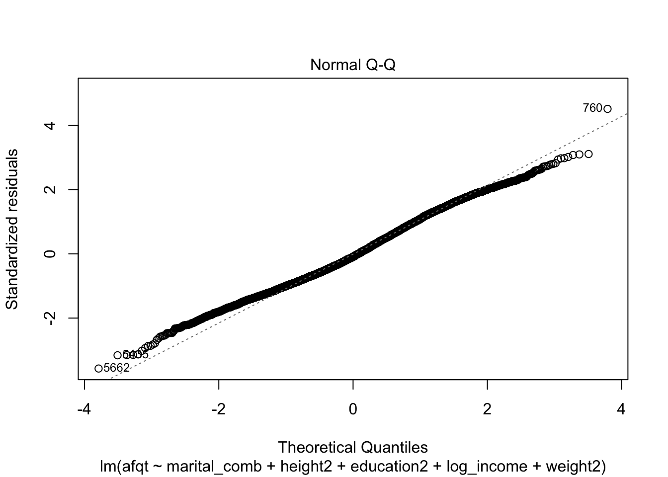
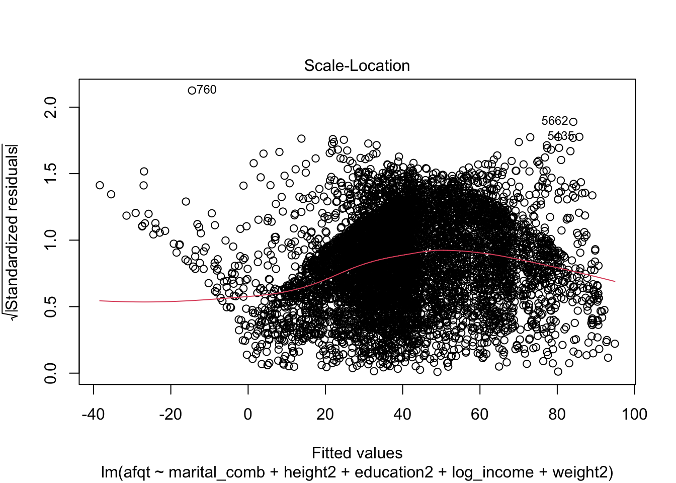
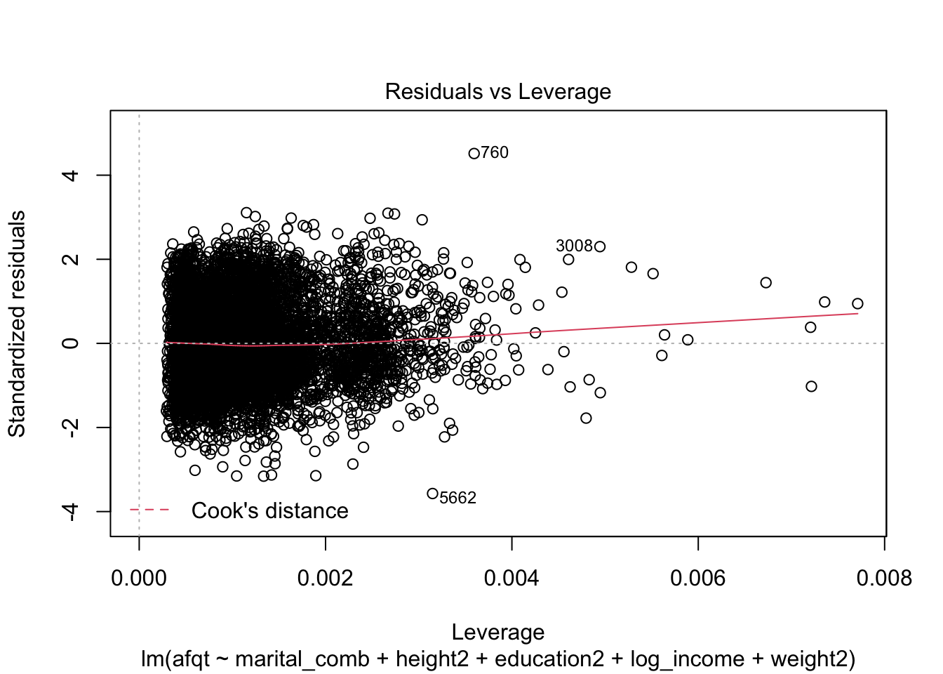
We could continue to model this variable by including additional predictors or interactions between our current predictors to attempt to remove this strong trend in the residuals. I’m going to stop here however and move on to another topic.
Exploring individual residuals
Evaluating all of the residuals in a single step using the plot function can be useful initially to explore model quality. However, eventually it is useful to explore residuals for specific values to explore why these are large.
There are a few options to do this, one uses the broom package, the other uses the modelr package. I show both below.
aug_afqt <- augment(afqt_alt)
aug_afqt
## # A tibble: 6,645 × 13
## .rownames afqt marital_comb height2 education2 log_income weight2 .fitted
## <chr> <dbl> <fct> <dbl> <dbl> <dbl> <dbl> <dbl>
## 1 1 6.84 married -7.10 -0.218 9.85 -33.3 39.9
## 2 2 49.4 married 2.90 -3.22 10.5 -32.3 30.2
## 3 3 99.4 married -2.10 2.78 11.6 6.70 61.1
## 4 4 44.0 married -4.10 0.782 10.6 8.70 47.3
## 5 5 59.7 married -1.10 0.782 11.2 1.70 50.1
## 6 6 98.8 divorced 0.896 4.78 11.5 11.7 70.6
## 7 7 82.3 married 6.90 2.78 -6.91 36.7 60.0
## 8 8 50.3 divorced -3.10 -1.22 11.2 -28.3 33.0
## 9 9 89.7 divorced 1.90 -1.22 11.0 -26.3 36.8
## 10 10 96.0 divorced 1.90 -0.218 11.9 5.70 42.2
## # … with 6,635 more rows, and 5 more variables: .resid <dbl>, .hat <dbl>,
## # .sigma <dbl>, .cooksd <dbl>, .std.resid <dbl>height_resid <- heights2 %>%
add_residuals(afqt_alt) %>%
add_predictions(afqt_alt)
height_resid## # A tibble: 7,006 × 16
## income height weight age marital sex education afqt marital_comb income2
## <int> <dbl> <int> <int> <fct> <fct> <int> <dbl> <fct> <dbl>
## 1 19000 60 155 53 married fema… 13 6.84 married 1.9 e+4
## 2 35000 70 156 51 married fema… 10 49.4 married 3.5 e+4
## 3 105000 65 195 52 married male 16 99.4 married 1.05e+5
## 4 40000 63 197 54 married fema… 14 44.0 married 4 e+4
## 5 75000 66 190 49 married male 14 59.7 married 7.5 e+4
## 6 102000 68 200 49 divorc… fema… 18 98.8 divorced 1.02e+5
## 7 0 74 225 48 married male 16 82.3 married 1 e-3
## 8 70000 64 160 54 divorc… fema… 12 50.3 divorced 7 e+4
## 9 60000 69 162 55 divorc… male 12 89.7 divorced 6 e+4
## 10 150000 69 194 54 divorc… male 13 96.0 divorced 1.5 e+5
## # … with 6,996 more rows, and 6 more variables: height2 <dbl>,
## # education2 <dbl>, weight2 <dbl>, log_income <dbl>, resid <dbl>, pred <dbl>The benefit to the augment function from the broom package is that it includes more information. The main benefit fo the add_residuals function from the modelr pacakge is that it includes all of the original data, not just those variables included in the final model. Therefore if you are fitting a model and want to explore trends in residuals based on other data characteristics not currently in the model, using the add_residuals function would likely be better for this use.
Filtering and Plotting Residuals
Now that we have these in a data frame, we could easily plot or filter residuals to explore cases in which the model is not adequatly fitting the dependent variable. For example, maybe we want to explore residuals greater than 50 in absolute value. This can easily be done with dplyr and the filter function.
filter(height_resid, abs(resid) > 50)## # A tibble: 113 × 16
## income height weight age marital sex education afqt marital_comb income2
## <int> <dbl> <int> <int> <fct> <fct> <int> <dbl> <fct> <dbl>
## 1 60000 69 162 55 divorc… male 12 89.7 divorced 6 e+4
## 2 150000 69 194 54 divorc… male 13 96.0 divorced 1.5e+5
## 3 45000 69 240 53 married male 12 98.8 married 4.5e+4
## 4 0 66 195 50 married fema… 14 99.2 married 1 e-3
## 5 93000 68 182 48 divorc… male 12 86.9 divorced 9.3e+4
## 6 43000 64 145 51 divorc… fema… 12 94.8 divorced 4.3e+4
## 7 52000 72 230 52 married male 12 93.1 married 5.2e+4
## 8 35000 59 165 49 divorc… fema… 12 80.0 divorced 3.5e+4
## 9 85000 61 140 55 married fema… 18 15.7 married 8.5e+4
## 10 0 69 186 55 separa… fema… 12 88.8 Other 1 e-3
## # … with 103 more rows, and 6 more variables: height2 <dbl>, education2 <dbl>,
## # weight2 <dbl>, log_income <dbl>, resid <dbl>, pred <dbl>You can also plot residuals directly or compared to other predictors.
ggplot(height_resid, aes(resid)) +
  geom_histogram() +
  theme_bw() +
  xlab("Residuals")
## `stat_bin()` using `bins = 30`. Pick better value with `binwidth`.## Warning: Removed 361 rows containing non-finite values (stat_bin).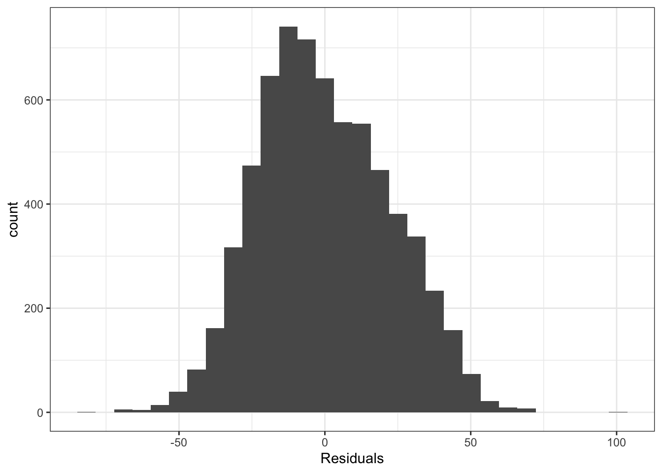
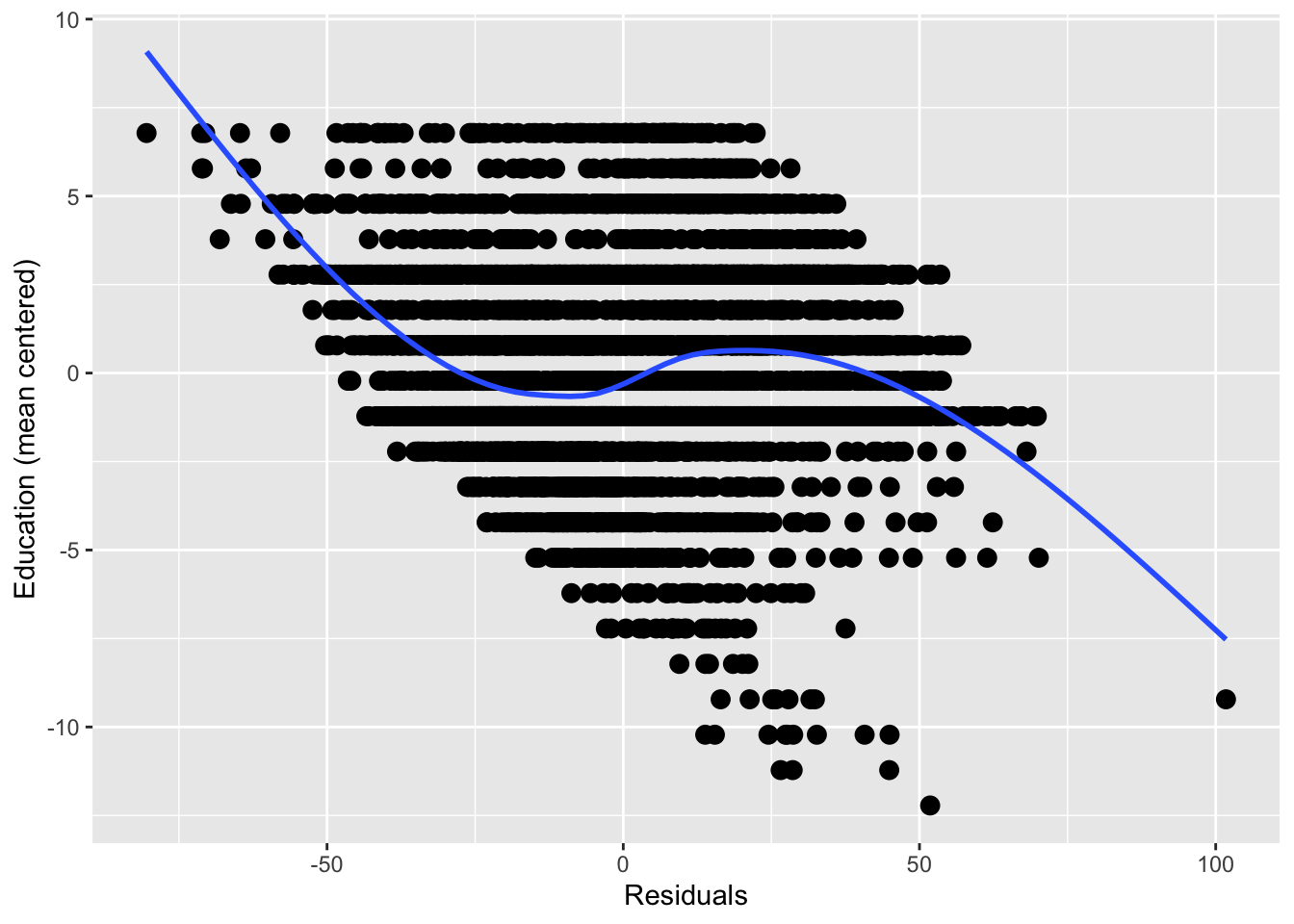
ggplot(height_resid, aes(resid, education2)) +
  geom_point(size = 3) +
  geom_smooth(size = 1, se = FALSE) +
  xlab("Residuals") +
  ylab("Education (mean centered)")
## `geom_smooth()` using method = 'gam' and formula 'y ~ s(x, bs = "cs")'## Warning: Removed 361 rows containing non-finite values (stat_smooth).## Warning: Removed 361 rows containing missing values (geom_point).