Model Introduction
This section of the notes is going to introduce you into the world of models in R. For the most part, we are going to stick with simple linear models and build up the various models using one function lm. The lm function is an extremely powerful function that can accommodate many different models in a single framework.
This section of notes is going to make use of four R packages:
library(tidyverse)
library(modelr)
# install.packages("broom")
library(broom)
library(fivethirtyeight)
Simple Linear Regression
First we need some data. We are going to explore the data from the fivethirtyeight package called fandango. Here are the first few rows:
fandango## # A tibble: 146 × 23
## film year rottentomatoes rottentomatoes_… metacritic metacritic_user imdb
## <chr> <dbl> <int> <int> <int> <dbl> <dbl>
## 1 Aveng… 2015 74 86 66 7.1 7.8
## 2 Cinde… 2015 85 80 67 7.5 7.1
## 3 Ant-M… 2015 80 90 64 8.1 7.8
## 4 Do Yo… 2015 18 84 22 4.7 5.4
## 5 Hot T… 2015 14 28 29 3.4 5.1
## 6 The W… 2015 63 62 50 6.8 7.2
## 7 Irrat… 2015 42 53 53 7.6 6.9
## 8 Top F… 2014 86 64 81 6.8 6.5
## 9 Shaun… 2015 99 82 81 8.8 7.4
## 10 Love … 2015 89 87 80 8.5 7.8
## # … with 136 more rows, and 16 more variables: fandango_stars <dbl>,
## # fandango_ratingvalue <dbl>, rt_norm <dbl>, rt_user_norm <dbl>,
## # metacritic_norm <dbl>, metacritic_user_nom <dbl>, imdb_norm <dbl>,
## # rt_norm_round <dbl>, rt_user_norm_round <dbl>, metacritic_norm_round <dbl>,
## # metacritic_user_norm_round <dbl>, imdb_norm_round <dbl>,
## # metacritic_user_vote_count <int>, imdb_user_vote_count <int>,
## # fandango_votes <int>, fandango_difference <dbl>These data have 146 rows and 23 columns.
Suppose we were interested in exploring the relationship between ratings from rottentomatoes and metacritic. Note, we will not use the user rating for this exploration. A natural first step may be to look at a scatterplot of these data to explore the shape of the relationship.
ggplot(fandango, aes(rottentomatoes, metacritic)) +
  theme_bw() +
  geom_point(size = 3)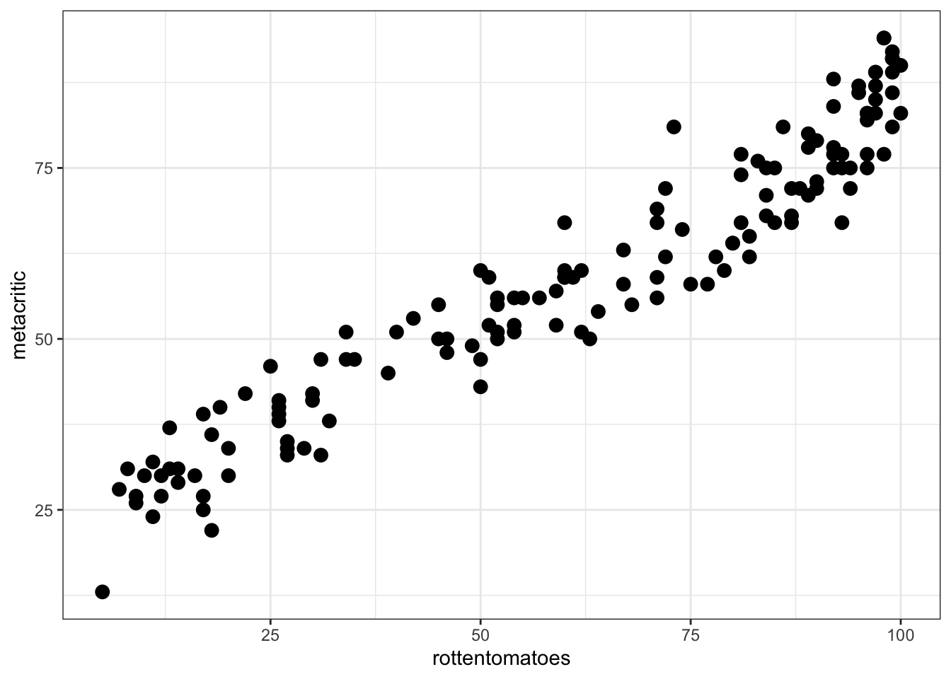
To better explore the relationship, including a smoother can be useful:
ggplot(fandango, aes(rottentomatoes, metacritic)) +
  theme_bw() +
  geom_point(size = 3) +
  geom_smooth(method = 'loess', se = FALSE, size = 1.5)
## `geom_smooth()` using formula 'y ~ x'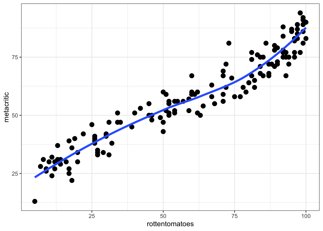
It may also be useful to calculate a correlation coefficient between these two variables.
with(fandango, cor(rottentomatoes, metacritic))## [1] 0.9573596Fit Linear Regression
Now we will attempt to fit a model to these data. Namely, the relationship appears to be mostly linear and suppose we wished to predict the metacritic review score with the rotten tomatoes score. To do this, we will use the lm function and the ~ that we used with facet_wrap and facet_grid.
More concretely, suppose we wished to fit the model: \[ metacritic_{i} = b_{0} + b_{1} rottentomatoes_{i} + \epsilon_{i} \]
In this model, \(metacritic_{i}\) is the dependent or response variable and \(rottentomatoes_{i}\) is the independent, predictor, or covariate. In many traditional statistics courses, \(metacritic_{i}\) would be represented with \(Y\) and \(rottentomatoes_{i}\) would be represented with \(X\). It is often more descriptive to represent these with their variable names instead of \(Y\) or \(X\).
To fit this model, we simply need to replace the \(=\) sign found in the equation above with the ~. For example, the equation above would turn into:
meta_mod <- lm(metacritic ~ rottentomatoes, data = fandango)To see output from the model, we can take two approaches. One is to use summary and another is to use the tidy function from the broom package. I show each below in turn.
summary(meta_mod)##
## Call:
## lm(formula = metacritic ~ rottentomatoes, data = fandango)
##
## Residuals:
## Min 1Q Median 3Q Max
## -11.7209 -4.1999 0.3855 3.7952 14.6662
##
## Coefficients:
## Estimate Std. Error t value Pr(>|t|)
## (Intercept) 21.12097 1.05710 19.98 <2e-16 ***
## rottentomatoes 0.61935 0.01558 39.77 <2e-16 ***
## ---
## Signif. codes: 0 '***' 0.001 '**' 0.01 '*' 0.05 '.' 0.1 ' ' 1
##
## Residual standard error: 5.658 on 144 degrees of freedom
## Multiple R-squared: 0.9165, Adjusted R-squared: 0.916
## F-statistic: 1581 on 1 and 144 DF, p-value: < 2.2e-16tidy(meta_mod)## # A tibble: 2 × 5
## term estimate std.error statistic p.value
## <chr> <dbl> <dbl> <dbl> <dbl>
## 1 (Intercept) 21.1 1.06 20.0 2.36e-43
## 2 rottentomatoes 0.619 0.0156 39.8 1.54e-79With the broom package, the results are reported in a tidier framework. We will see additional useful functions using the broom package later on.
You can also directly request confidence intervals with the tidy function:
tidy(meta_mod, conf.int = TRUE)## # A tibble: 2 × 7
## term estimate std.error statistic p.value conf.low conf.high
## <chr> <dbl> <dbl> <dbl> <dbl> <dbl> <dbl>
## 1 (Intercept) 21.1 1.06 20.0 2.36e-43 19.0 23.2
## 2 rottentomatoes 0.619 0.0156 39.8 1.54e-79 0.589 0.650Exercises
- Fit a new model using the
fandangodata that attempts to explain the metacritic ratings with the imdb rating. - Fit another model using the
fandangodata that attempts to explain the metacritic ratings with the fandango_ratingvalue scores. - Exploring the predictors of these two new models with the one fitted above with the rottentomatoes scores, which rating score best helps us predict the metacritic scores?
Workings Behind lm function
To see what the lm function is doing behind the scenes, we will use the model_matrix function from the modelr package. For example, from the model above:
model_matrix(fandango, metacritic ~ rottentomatoes)## # A tibble: 146 × 2
## `(Intercept)` rottentomatoes
## <dbl> <dbl>
## 1 1 74
## 2 1 85
## 3 1 80
## 4 1 18
## 5 1 14
## 6 1 63
## 7 1 42
## 8 1 86
## 9 1 99
## 10 1 89
## # … with 136 more rowsThis is often referred to as the design matrix in statistics text books and is one of the matrices that are used by lm to calculate the estimated parameters from above. Notice that is automatically included the intercept, normally this is of interest, if it is not, we can omit it directly by including a -1 in the formula. For example:
model_matrix(fandango, metacritic ~ rottentomatoes - 1)## # A tibble: 146 × 1
## rottentomatoes
## <dbl>
## 1 74
## 2 85
## 3 80
## 4 18
## 5 14
## 6 63
## 7 42
## 8 86
## 9 99
## 10 89
## # … with 136 more rowstidy(lm(metacritic ~ rottentomatoes - 1, data = fandango))## # A tibble: 1 × 5
## term estimate std.error statistic p.value
## <chr> <dbl> <dbl> <dbl> <dbl>
## 1 rottentomatoes 0.898 0.0134 67.3 3.14e-111You need to be careful with this syntax as this is commonly not is what is desired when fitting a linear model.
Categorical Predictors
Suppose we were interested in the following research question:
- To what extent are there average differences in movie ratings between rottentomatoes and metacritic?
To answer this research question, we would need to transform our data to great a group variable and a rating variable.
meta_rotten <- fandango %>%
  select(film, year, rottentomatoes, metacritic) %>%
  gather(group, rating, rottentomatoes, metacritic)
meta_rotten
## # A tibble: 292 × 4
## film year group rating
## <chr> <dbl> <chr> <int>
## 1 Avengers: Age of Ultron 2015 rottentomatoes 74
## 2 Cinderella 2015 rottentomatoes 85
## 3 Ant-Man 2015 rottentomatoes 80
## 4 Do You Believe? 2015 rottentomatoes 18
## 5 Hot Tub Time Machine 2 2015 rottentomatoes 14
## 6 The Water Diviner 2015 rottentomatoes 63
## 7 Irrational Man 2015 rottentomatoes 42
## 8 Top Five 2014 rottentomatoes 86
## 9 Shaun the Sheep Movie 2015 rottentomatoes 99
## 10 Love & Mercy 2015 rottentomatoes 89
## # … with 282 more rowsNow we can work with this data to answer the question from above. More specifically, our dependent variable will be the rating variable and the independent variable will be the group (categorical) variable. This can be fitted within a linear model as follows:
tidy(lm(rating ~ factor(group), data = meta_rotten))## # A tibble: 2 × 5
## term estimate std.error statistic p.value
## <chr> <dbl> <dbl> <dbl> <dbl>
## 1 (Intercept) 58.8 2.10 28.0 2.50e-84
## 2 factor(group)rottentomatoes 2.04 2.97 0.686 4.93e- 1To see exactly what is happening, model_matrix may be useful. First I am going to arrange the data by the films in alphabetical order.
meta_rotten %>%
  arrange(film)
## # A tibble: 292 × 4
## film year group rating
## <chr> <dbl> <chr> <int>
## 1 '71 2015 rottentomatoes 97
## 2 '71 2015 metacritic 83
## 3 5 Flights Up 2015 rottentomatoes 52
## 4 5 Flights Up 2015 metacritic 55
## 5 A Little Chaos 2015 rottentomatoes 40
## 6 A Little Chaos 2015 metacritic 51
## 7 A Most Violent Year 2014 rottentomatoes 90
## 8 A Most Violent Year 2014 metacritic 79
## 9 About Elly 2015 rottentomatoes 97
## 10 About Elly 2015 metacritic 87
## # … with 282 more rowsmeta_rotten %>%
arrange(film) %>%
model_matrix(rating ~ factor(group))## # A tibble: 292 × 2
## `(Intercept)` `factor(group)rottentomatoes`
## <dbl> <dbl>
## 1 1 1
## 2 1 0
## 3 1 1
## 4 1 0
## 5 1 1
## 6 1 0
## 7 1 1
## 8 1 0
## 9 1 1
## 10 1 0
## # … with 282 more rowsYou may be more familiar with using a t-test for this type of design. We can replicate the results above with a t-test using the t.test function.
t.test(rating ~ factor(group), data = meta_rotten,
       var.equal = TRUE)
##
## Two Sample t-test
##
## data: rating by factor(group)
## t = -0.68638, df = 290, p-value = 0.493
## alternative hypothesis: true difference in means between group metacritic and group rottentomatoes is not equal to 0
## 95 percent confidence interval:
## -7.893918 3.811726
## sample estimates:
## mean in group metacritic mean in group rottentomatoes
## 58.80822 60.84932Exercises
- Compute descriptive means using the
meta_rottentransformed data from above by the group variable. Do these means appear to be descriptively different? - How do these means relate to the parameters estimated from the model above?
Evaulating Model fit
There are many ways to evaluate model fit. Many of these are available using the summary function.
summary(lm(rating ~ factor(group), data = meta_rotten))##
## Call:
## lm(formula = rating ~ factor(group), data = meta_rotten)
##
## Residuals:
## Min 1Q Median 3Q Max
## -55.849 -19.089 0.671 22.161 39.151
##
## Coefficients:
## Estimate Std. Error t value Pr(>|t|)
## (Intercept) 58.808 2.103 27.967 <2e-16 ***
## factor(group)rottentomatoes 2.041 2.974 0.686 0.493
## ---
## Signif. codes: 0 '***' 0.001 '**' 0.01 '*' 0.05 '.' 0.1 ' ' 1
##
## Residual standard error: 25.41 on 290 degrees of freedom
## Multiple R-squared: 0.001622, Adjusted R-squared: -0.001821
## F-statistic: 0.4711 on 1 and 290 DF, p-value: 0.493The unfortunate part of this is the fact that these are more difficult to pull out of the table programmatically (i.e. in a reproducible workflow). This is where the broom package helps with the use of the glance function.
glance(lm(rating ~ factor(group), data = meta_rotten))## # A tibble: 1 × 12
## r.squared adj.r.squared sigma statistic p.value df logLik AIC BIC
## <dbl> <dbl> <dbl> <dbl> <dbl> <dbl> <dbl> <dbl> <dbl>
## 1 0.00162 -0.00182 25.4 0.471 0.493 1 -1358. 2722. 2733.
## # … with 3 more variables: deviance <dbl>, df.residual <int>, nobs <int>These are now in a more tidy data frame and if you have multiple models in an exploratory analysis, these could then be much easier compared and combined programmatically to come to a final model.
Another useful function from the broom package is augment. This function will add additional information to the original data such as residuals, fitted (predicted) values, and other diagnostic statistics.
diagnostic <- augment(lm(rating ~ factor(group), data = meta_rotten))
diagnostic
## # A tibble: 292 × 7
## rating `factor(group)` .fitted .hat .sigma .cooksd .std.resid
## <int> <fct> <dbl> <dbl> <dbl> <dbl> <dbl>
## 1 74 rottentomatoes 60.8 0.00685 25.4 0.000930 0.519
## 2 85 rottentomatoes 60.8 0.00685 25.4 0.00314 0.954
## 3 80 rottentomatoes 60.8 0.00685 25.4 0.00197 0.756
## 4 18 rottentomatoes 60.8 0.00685 25.3 0.00988 -1.69
## 5 14 rottentomatoes 60.8 0.00685 25.3 0.0118 -1.85
## 6 63 rottentomatoes 60.8 0.00685 25.5 0.0000249 0.0849
## 7 42 rottentomatoes 60.8 0.00685 25.4 0.00191 -0.744
## 8 86 rottentomatoes 60.8 0.00685 25.4 0.00340 0.993
## 9 99 rottentomatoes 60.8 0.00685 25.4 0.00783 1.51
## 10 89 rottentomatoes 60.8 0.00685 25.4 0.00426 1.11
## # … with 282 more rowsThese could then be plotted to explore more information about model fit. For example a histogram of the standardized residuals are often useful.
ggplot(diagnostic, aes(.std.resid)) +
  geom_histogram(bins = 30, color = 'white') +
  theme_bw()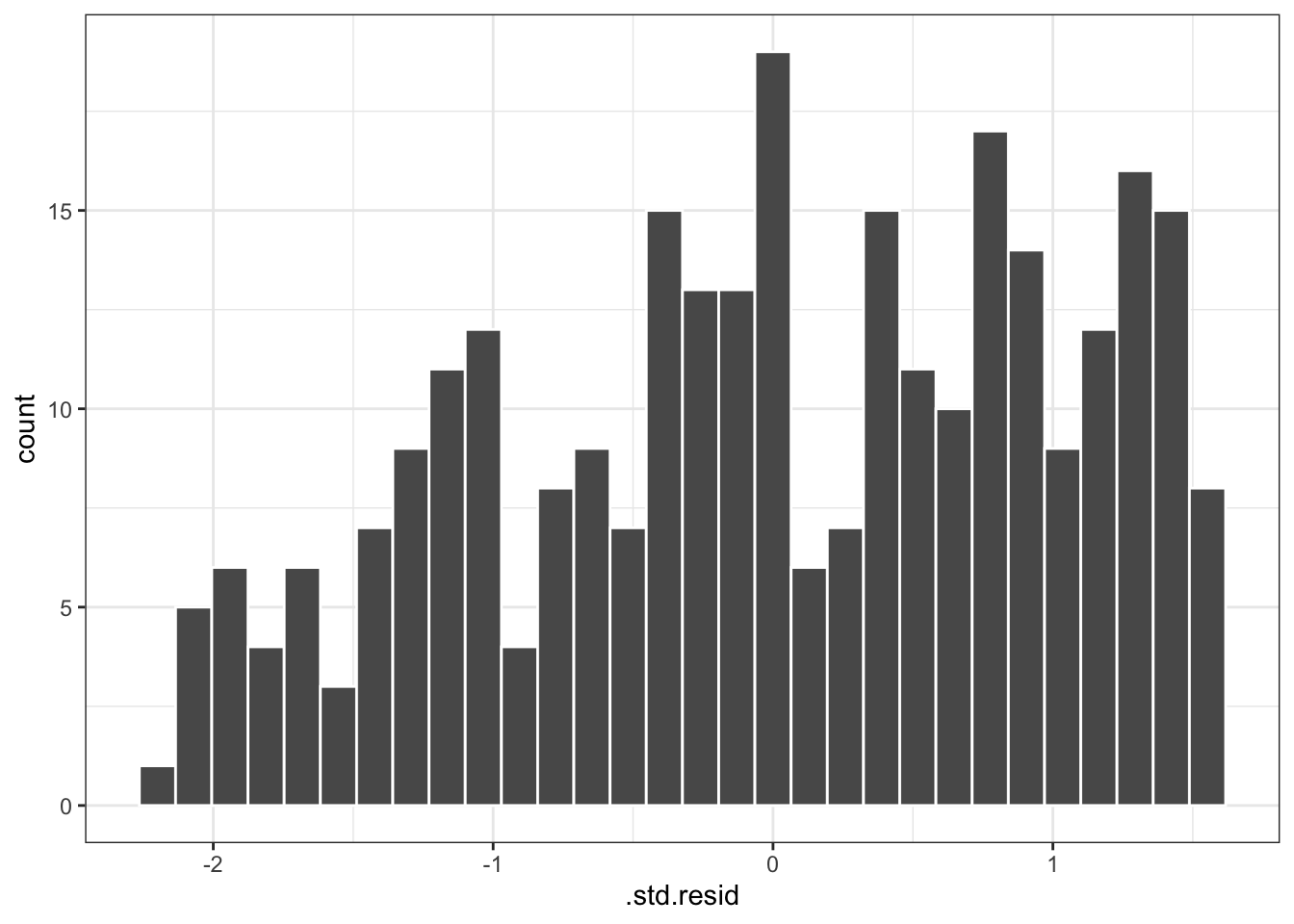
For this model, boxplots of the standardized residuals by the two groups can also be informative:
ggplot(diagnostic, aes(`factor(group)`, .std.resid)) +
  geom_boxplot() +
  geom_jitter() +
  coord_flip() +
  theme_bw()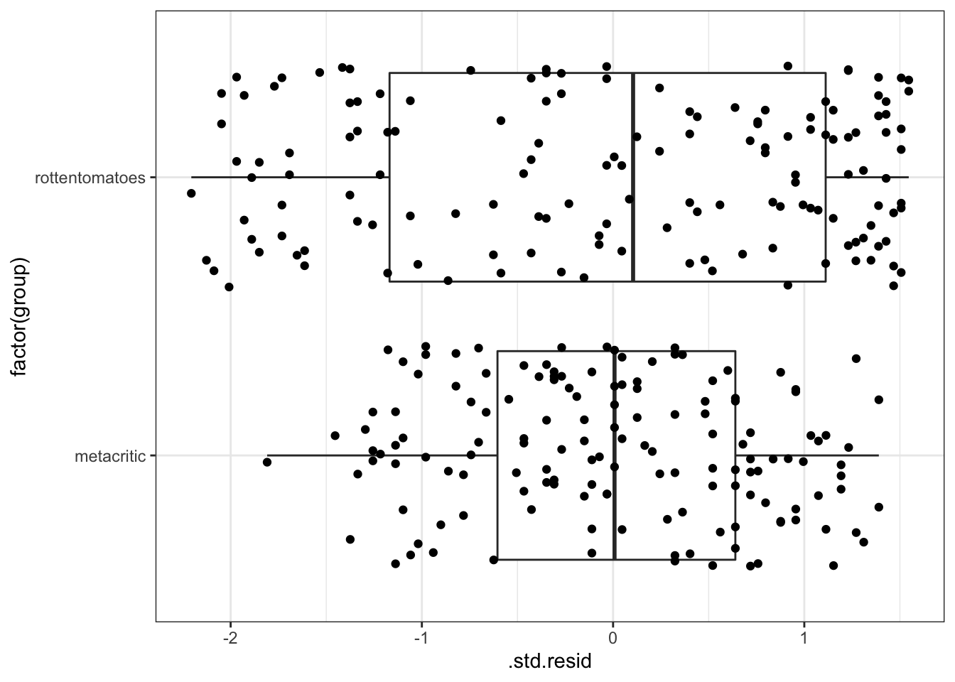
We will explore more details on predicted or fitted values later.
Lastly, the augment function can be useful, however I personally do not like the naming convention used by the function. I want to point you to two additional functions from the modelr package that can be useful for predicted (add_predictions) and residual values (add_residuals).
For example, to add the residuals to the original data:
meta_rotten %>%
  add_residuals(lm(rating ~ factor(group), data = meta_rotten))
## # A tibble: 292 × 5
## film year group rating resid
## <chr> <dbl> <chr> <int> <dbl>
## 1 Avengers: Age of Ultron 2015 rottentomatoes 74 13.2
## 2 Cinderella 2015 rottentomatoes 85 24.2
## 3 Ant-Man 2015 rottentomatoes 80 19.2
## 4 Do You Believe? 2015 rottentomatoes 18 -42.8
## 5 Hot Tub Time Machine 2 2015 rottentomatoes 14 -46.8
## 6 The Water Diviner 2015 rottentomatoes 63 2.15
## 7 Irrational Man 2015 rottentomatoes 42 -18.8
## 8 Top Five 2014 rottentomatoes 86 25.2
## 9 Shaun the Sheep Movie 2015 rottentomatoes 99 38.2
## 10 Love & Mercy 2015 rottentomatoes 89 28.2
## # … with 282 more rowsExercises
- Fit a new model using the
fandangodata that attempts to explain the metacritic ratings with the imdb rating. Explore the distribution of residuals. Does there appear to be problems with these residuals? - Using the model from #1, create a scatterplot that displays the residuals by the predictor variable. Are there problems with this plot that we should be concerned with?