Building Upon Linear Models
The last week has focused on building simple linear models with a single predictor. This week will evaluate these models and build them up with more complexity. Particularly, this week will focus on ways to build models with predictors that have more than two categories, alternative ways to code categorical predictors, mixing categorical and quantitative variables, and interactions.
This section of notes will use the following packages.
library(tidyverse)
library(modelr)
library(broom)
library(fivethirtyeight)
library(forcats)
More than two categorical levels
Last week we explored a linear model framework for a two sample t-test (and the homework has you explore fitting a one-sample t-test in a linear model framework). I now want to generalize this idea to more than two categorical levels. It is traditional to think about these types of models as analysis of variance (ANOVA) models, however, the same model can be fitted in a linear model framework as well.
For this set of notes, we are going to make use of the gss_cat data found in the forcats package. Below are the first few rows of the data:
gss_cat## # A tibble: 21,483 × 9
## year marital age race rincome partyid relig denom tvhours
## <int> <fct> <int> <fct> <fct> <fct> <fct> <fct> <int>
## 1 2000 Never married 26 White $8000 to 9999 Ind,near … Prot… Sout… 12
## 2 2000 Divorced 48 White $8000 to 9999 Not str r… Prot… Bapt… NA
## 3 2000 Widowed 67 White Not applicable Independe… Prot… No d… 2
## 4 2000 Never married 39 White Not applicable Ind,near … Orth… Not … 4
## 5 2000 Divorced 25 White Not applicable Not str d… None Not … 1
## 6 2000 Married 25 White $20000 - 24999 Strong de… Prot… Sout… NA
## 7 2000 Never married 36 White $25000 or more Not str r… Chri… Not … 3
## 8 2000 Divorced 44 White $7000 to 7999 Ind,near … Prot… Luth… NA
## 9 2000 Married 44 White $25000 or more Not str d… Prot… Other 0
## 10 2000 Married 47 White $25000 or more Strong re… Prot… Sout… 3
## # … with 21,473 more rowsSuppose we were interested in exploring the relationship between the marital status of an individual and how much tv they watch. For example, perhaps married couples watch more tv compared to those that are single or never married. To get an idea of the categories in the marital variable, we could use the count function within dplyr.
gss_cat %>%
  count(marital)
## # A tibble: 6 × 2
## marital n
## <fct> <int>
## 1 No answer 17
## 2 Never married 5416
## 3 Separated 743
## 4 Divorced 3383
## 5 Widowed 1807
## 6 Married 10117You’ll notice that there a few responses of “No Answer” and we may wish to treat these as missing values. This can be done with the fct_recode function as follows:
gss_cat <- gss_cat %>%
  mutate(marital_miss = fct_recode(marital,
    NULL = 'No answer'
  ))
gss_cat %>%
  count(marital_miss)
## # A tibble: 6 × 2
## marital_miss n
## <fct> <int>
## 1 Never married 5416
## 2 Separated 743
## 3 Divorced 3383
## 4 Widowed 1807
## 5 Married 10117
## 6 <NA> 17We can now fit the model to this new data using the lm function.
anova_mod <- lm(tvhours ~ marital_miss, data = gss_cat)
summary(anova_mod)
##
## Call:
## lm(formula = tvhours ~ marital_miss, data = gss_cat)
##
## Residuals:
## Min 1Q Median 3Q Max
## -3.9120 -1.6504 -0.6504 0.8948 21.3496
##
## Coefficients:
## Estimate Std. Error t value Pr(>|t|)
## (Intercept) 3.10518 0.04679 66.366 < 2e-16 ***
## marital_missSeparated 0.44444 0.13738 3.235 0.00122 **
## marital_missDivorced -0.01977 0.07680 -0.257 0.79687
## marital_missWidowed 0.80682 0.09352 8.627 < 2e-16 ***
## marital_missMarried -0.45475 0.05879 -7.735 1.13e-14 ***
## ---
## Signif. codes: 0 '***' 0.001 '**' 0.01 '*' 0.05 '.' 0.1 ' ' 1
##
## Residual standard error: 2.561 on 11323 degrees of freedom
## (10155 observations deleted due to missingness)
## Multiple R-squared: 0.02141, Adjusted R-squared: 0.02107
## F-statistic: 61.94 on 4 and 11323 DF, p-value: < 2.2e-16To explore what the lm function is doing internally, the design matrix is a natural way to do this.
model_matrix(gss_cat, tvhours ~ marital_miss)## # A tibble: 11,328 × 5
## `(Intercept)` marital_missSeparated marital_missDivorced marital_missWidowed
## <dbl> <dbl> <dbl> <dbl>
## 1 1 0 0 0
## 2 1 0 0 1
## 3 1 0 0 0
## 4 1 0 1 0
## 5 1 0 0 0
## 6 1 0 0 0
## 7 1 0 0 0
## 8 1 0 0 0
## 9 1 0 0 0
## 10 1 0 1 0
## # … with 11,318 more rows, and 1 more variable: marital_missMarried <dbl>Writing out this model with equations, the model looks like this: \[ tvhours_{i} = \beta_{0} + \beta_{1} Separated_{i} + \beta_{2} Divorced_{I} + \beta_{3} Widowed_{i} + \beta_{4} Married_{i} + \epsilon_{i} \]
If you are more familiar with ANOVA terminology, you can get an ANOVA table using the anova function on the model object.
anova(anova_mod)## Analysis of Variance Table
##
## Response: tvhours
## Df Sum Sq Mean Sq F value Pr(>F)
## marital_miss 4 1624 406.12 61.941 < 2.2e-16 ***
## Residuals 11323 74239 6.56
## ---
## Signif. codes: 0 '***' 0.001 '**' 0.01 '*' 0.05 '.' 0.1 ' ' 1Here you’ll notice that the F statistic is the same from the lm and anova functions showing that these are equivalent model calls.
Exercises
- Using the martial_miss variable created above, what are the sample means of the five groups?
- How do these sample means relate back to the parameters estimates shown above?
- How could you visualize these models results? Attempt to create a visualization that captures the model results above.
Adjusting the reference group
It is often of interest to adjust the reference group to make the intercept represent a specific group of interest. There are two approaches to take for this approach. The first I will show is using the forcats package to change the order of the levels of the variable.
Suppose for example, we wish to make the widowed category the reference group. This is the job of fct_relevel from the forcats package.
gss_cat <- gss_cat %>%
  mutate(marital_m_widow = fct_relevel(
    marital_miss,
    'Widowed'
  ))
levels(gss_cat$marital_miss)
## [1] "Never married" "Separated" "Divorced" "Widowed"
## [5] "Married"levels(gss_cat$marital_m_widow)## [1] "Widowed" "Never married" "Separated" "Divorced"
## [5] "Married"You’ll notice that in the new variable, the widowed category was moved to the beginning and the remaining order was not changed. We can now fit a new model with this newly releveled factor variable.
summary(lm(tvhours ~ marital_m_widow, data = gss_cat))##
## Call:
## lm(formula = tvhours ~ marital_m_widow, data = gss_cat)
##
## Residuals:
## Min 1Q Median 3Q Max
## -3.9120 -1.6504 -0.6504 0.8948 21.3496
##
## Coefficients:
## Estimate Std. Error t value Pr(>|t|)
## (Intercept) 3.91200 0.08097 48.313 < 2e-16 ***
## marital_m_widowNever married -0.80682 0.09352 -8.627 < 2e-16 ***
## marital_m_widowSeparated -0.36238 0.15245 -2.377 0.0175 *
## marital_m_widowDivorced -0.82659 0.10132 -8.159 3.75e-16 ***
## marital_m_widowMarried -1.26157 0.08845 -14.262 < 2e-16 ***
## ---
## Signif. codes: 0 '***' 0.001 '**' 0.01 '*' 0.05 '.' 0.1 ' ' 1
##
## Residual standard error: 2.561 on 11323 degrees of freedom
## (10155 observations deleted due to missingness)
## Multiple R-squared: 0.02141, Adjusted R-squared: 0.02107
## F-statistic: 61.94 on 4 and 11323 DF, p-value: < 2.2e-16The second approach to modifying which group represents the reference group would be to create the indicator (dummy) variables manually. The logic follows from the design matrix above, namely that each variable should have a value of 1 if the marital status equals a specific category or 0 otherwise. For example, this can be created as follows:
gss_cat <- gss_cat %>%
  mutate(
    separated = ifelse(marital_miss == 'Separated', 1, 0),
    never_married = ifelse(marital_miss == 'Never married', 1, 0),
    divorced = ifelse(marital_miss == 'Divorced', 1, 0),
    married = ifelse(marital_miss == 'Married', 1, 0)
  )
summary(lm(tvhours ~ separated + never_married + divorced + married,
           data = gss_cat))
##
## Call:
## lm(formula = tvhours ~ separated + never_married + divorced +
## married, data = gss_cat)
##
## Residuals:
## Min 1Q Median 3Q Max
## -3.9120 -1.6504 -0.6504 0.8948 21.3496
##
## Coefficients:
## Estimate Std. Error t value Pr(>|t|)
## (Intercept) 3.91200 0.08097 48.313 < 2e-16 ***
## separated -0.36238 0.15245 -2.377 0.0175 *
## never_married -0.80682 0.09352 -8.627 < 2e-16 ***
## divorced -0.82659 0.10132 -8.159 3.75e-16 ***
## married -1.26157 0.08845 -14.262 < 2e-16 ***
## ---
## Signif. codes: 0 '***' 0.001 '**' 0.01 '*' 0.05 '.' 0.1 ' ' 1
##
## Residual standard error: 2.561 on 11323 degrees of freedom
## (10155 observations deleted due to missingness)
## Multiple R-squared: 0.02141, Adjusted R-squared: 0.02107
## F-statistic: 61.94 on 4 and 11323 DF, p-value: < 2.2e-16Manually creating the variables has a few advantages, namely that there is a bit more flexibility on how the variables are created, but both approaches lead to the same model.
Exercises
- Combine the ‘Never married’ and ‘Divorced’ categories into one category.
- Fit a new model that combines these two categories. Does the model fit differ from the models shown above? Is this surprising?
Post Hoc Tests
From the models fitted above, it may be of interest to conduct post hoc tests that compare all pairwise mean differences, particularly as the tests above are all compared to the reference group. This approach will be explored using the multcomp package and with defining linear contrasts.
# install.packages("multcomp")
library(multcomp)
We first need to define linear contrasts based on the levels of the factor variable. For example, using the following model:
gss_cat <- gss_cat %>%
  mutate(marital_m_widow = fct_recode(marital_m_widow,
           "Never_married" = "Never married"
  ))
anova_mod <- lm(tvhours ~ marital_m_widow, data = gss_cat)
levels(gss_cat$marital_m_widow)
## [1] "Widowed" "Never_married" "Separated" "Divorced"
## [5] "Married"We will use these level values to create linear contrasts that test all pairwise categories.
my_contrasts <- c("Widowed - Never_married = 0",
                 "Widowed - Separated = 0",
                 "Widowed - Divorced = 0",
                 "Widowed - Married = 0",
                 "Never_married - Separated = 0",
                 "Never_married - Divorced = 0",
                 "Never_married - Married = 0",
                 "Separated - Divorced = 0",
                 "Separated - Married = 0",
                 "Divorced - Married = 0")
contr_results <- glht(anova_mod,
                      linfct = mcp(marital_m_widow = my_contrasts))
summary(contr_results)
##
## Simultaneous Tests for General Linear Hypotheses
##
## Multiple Comparisons of Means: User-defined Contrasts
##
##
## Fit: lm(formula = tvhours ~ marital_m_widow, data = gss_cat)
##
## Linear Hypotheses:
## Estimate Std. Error t value Pr(>|t|)
## Widowed - Never_married == 0 0.80682 0.09352 8.627 < 0.001 ***
## Widowed - Separated == 0 0.36238 0.15245 2.377 0.11076
## Widowed - Divorced == 0 0.82659 0.10132 8.159 < 0.001 ***
## Widowed - Married == 0 1.26157 0.08845 14.262 < 0.001 ***
## Never_married - Separated == 0 -0.44444 0.13738 -3.235 0.00957 **
## Never_married - Divorced == 0 0.01977 0.07680 0.257 0.99893
## Never_married - Married == 0 0.45475 0.05879 7.735 < 0.001 ***
## Separated - Divorced == 0 0.46421 0.14280 3.251 0.00904 **
## Separated - Married == 0 0.89919 0.13398 6.711 < 0.001 ***
## Divorced - Married == 0 0.43498 0.07054 6.166 < 0.001 ***
## ---
## Signif. codes: 0 '***' 0.001 '**' 0.01 '*' 0.05 '.' 0.1 ' ' 1
## (Adjusted p values reported -- single-step method)You can also specify different adjustment methods, such as the Benjamin-Hochberg method.
summary(contr_results, test = adjusted("BH"))##
## Simultaneous Tests for General Linear Hypotheses
##
## Multiple Comparisons of Means: User-defined Contrasts
##
##
## Fit: lm(formula = tvhours ~ marital_m_widow, data = gss_cat)
##
## Linear Hypotheses:
## Estimate Std. Error t value Pr(>|t|)
## Widowed - Never_married == 0 0.80682 0.09352 8.627 < 2e-16 ***
## Widowed - Separated == 0 0.36238 0.15245 2.377 0.01941 *
## Widowed - Divorced == 0 0.82659 0.10132 8.159 1.48e-15 ***
## Widowed - Married == 0 1.26157 0.08845 14.262 < 2e-16 ***
## Never_married - Separated == 0 -0.44444 0.13738 -3.235 0.00152 **
## Never_married - Divorced == 0 0.01977 0.07680 0.257 0.79687
## Never_married - Married == 0 0.45475 0.05879 7.735 2.78e-14 ***
## Separated - Divorced == 0 0.46421 0.14280 3.251 0.00152 **
## Separated - Married == 0 0.89919 0.13398 6.711 4.04e-11 ***
## Divorced - Married == 0 0.43498 0.07054 6.166 1.20e-09 ***
## ---
## Signif. codes: 0 '***' 0.001 '**' 0.01 '*' 0.05 '.' 0.1 ' ' 1
## (Adjusted p values reported -- BH method)Although defining the linear contrasts manually is more flexible, for simple models, the multiple comparisons can be generated a bit more simply.
summary(glht(anova_mod, linfct = mcp(marital_m_widow = "Tukey")),
        test = adjusted("BH"))
##
## Simultaneous Tests for General Linear Hypotheses
##
## Multiple Comparisons of Means: Tukey Contrasts
##
##
## Fit: lm(formula = tvhours ~ marital_m_widow, data = gss_cat)
##
## Linear Hypotheses:
## Estimate Std. Error t value Pr(>|t|)
## Never_married - Widowed == 0 -0.80682 0.09352 -8.627 < 2e-16 ***
## Separated - Widowed == 0 -0.36238 0.15245 -2.377 0.01941 *
## Divorced - Widowed == 0 -0.82659 0.10132 -8.159 1.48e-15 ***
## Married - Widowed == 0 -1.26157 0.08845 -14.262 < 2e-16 ***
## Separated - Never_married == 0 0.44444 0.13738 3.235 0.00152 **
## Divorced - Never_married == 0 -0.01977 0.07680 -0.257 0.79687
## Married - Never_married == 0 -0.45475 0.05879 -7.735 2.78e-14 ***
## Divorced - Separated == 0 -0.46421 0.14280 -3.251 0.00152 **
## Married - Separated == 0 -0.89919 0.13398 -6.711 4.04e-11 ***
## Married - Divorced == 0 -0.43498 0.07054 -6.166 1.20e-09 ***
## ---
## Signif. codes: 0 '***' 0.001 '**' 0.01 '*' 0.05 '.' 0.1 ' ' 1
## (Adjusted p values reported -- BH method)You can also generate simultaneous confidence intervals:
ci <- confint(summary(glht(anova_mod, linfct = mcp(marital_m_widow = "Tukey")),
                test = adjusted("BH")))
ci
##
## Simultaneous Confidence Intervals
##
## Multiple Comparisons of Means: Tukey Contrasts
##
##
## Fit: lm(formula = tvhours ~ marital_m_widow, data = gss_cat)
##
## Quantile = 2.6895
## 95% family-wise confidence level
##
##
## Linear Hypotheses:
## Estimate lwr upr
## Never_married - Widowed == 0 -0.80682 -1.05834 -0.55531
## Separated - Widowed == 0 -0.36238 -0.77239 0.04762
## Divorced - Widowed == 0 -0.82659 -1.09908 -0.55410
## Married - Widowed == 0 -1.26157 -1.49947 -1.02367
## Separated - Never_married == 0 0.44444 0.07497 0.81392
## Divorced - Never_married == 0 -0.01977 -0.22631 0.18678
## Married - Never_married == 0 -0.45475 -0.61288 -0.29662
## Divorced - Separated == 0 -0.46421 -0.84827 -0.08015
## Married - Separated == 0 -0.89919 -1.25954 -0.53885
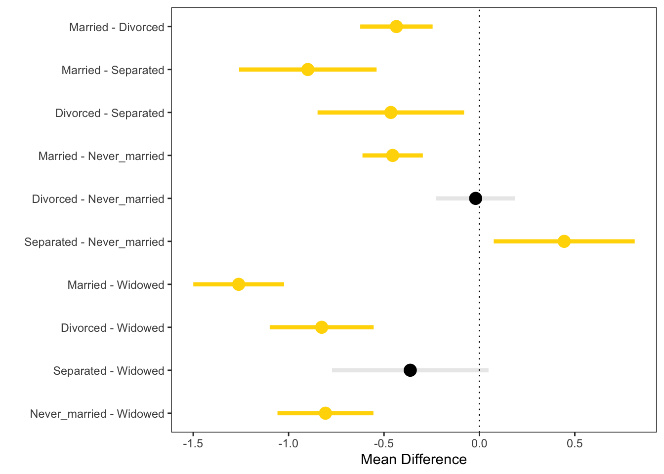
## Married - Divorced == 0 -0.43498 -0.62471 -0.24526These could then be visulized directly.
SCI = data.frame(
  Contrast = 1:nrow(ci$confint),   #Contrast number
  MD = ci$confint[, 1],      #Mean difference
  LL = ci$confint[, 2],      #Lower limit
  UL = ci$confint[, 3],      #Upper limit
  Sig = c("Yes", "No", "Yes", "Yes", 'Yes', 'No',
          'Yes', 'Yes', 'Yes', 'Yes'),   #Statistically reliable?
  Alpha = c(1, .75, 1, 1, 1, .75, 1, 1, 1, 1),     #Transparency value
  Names = rownames(ci$confint)  # contrast label
)

# Plot of the simultaneous intervals
library(ggplot2)
ggplot(data = SCI, aes(x = Contrast, y = MD, color = Sig)) +
  geom_point(size = 4) +
  geom_segment(aes(x = Contrast, xend = Contrast, y = LL,
                   yend = UL, alpha = Alpha), lwd = 1.5) +
  geom_hline(yintercept = 0, lty = "dotted") +
  scale_color_manual(values = c("Black", "Gold")) +
  scale_x_continuous(
    name = "",
    breaks = 1:10,
    labels = SCI$Names
  ) +
  ylab("Mean Difference") +
  coord_flip() +
  theme_bw() +
  theme(
    legend.position = "none",
    panel.grid.minor = element_blank(),
    panel.grid.major = element_blank()
  )
Exercises
- Fit a model that explores mean differences in tvhours by the party affiliation (partyid variable). Do the means differ?
- Using the post-hoc tests, run post-hoc tests to test all pairwise differences.